Dual-targeted bicistronic CAR-T-cell therapy (Su 2025)
Source:vignettes/articles/Su_2025_dual_targeted_cart.Rmd
Su_2025_dual_targeted_cart.RmdModel and source
Su et al. developed a multiscale mechanistic cellular-kinetic / pharmacodynamic (CK-PD) framework for dual-targeted bicistronic CAR T-cell therapy, in which a single T cell expresses two independent chimeric-antigen receptors. The paper builds the framework in two layers and validates it on two antigen pairs:
- An in vitro cell-level tumour-killing model (Figure 1a) in which CAR T cells and tumour cells coexist in a culture well, the two CARs form single- and double-target complexes, and complexes per tumour cell drive Emax killing. It is fit to CD19/CD22 CAR-T co-cultured with B-cell ALL cell lines and validated on an independent GPRC5D/BCMA CAR-T multiple-myeloma dataset whose two co-stimulatory-domain designs are compared.
- An in vivo clinical CK-PD model (Figure 1b) that embeds the same binding and killing mechanism in a two-compartment (peripheral blood + bone marrow) cellular-kinetic structure with effector/memory phenotype transformation, and fits it to the phase 1 CD19/CD22 CAR-T (AUTO3) dose-escalation study in pediatric and young-adult B-ALL.
This article packages four model files from the paper:
mod_clin <- readModelDb("Su_2025_cd19cd22cart_ALL")
mod_vitro_ball <- readModelDb("Su_2025_cd19cd22cart_invitro")
mod_vitro_41bb <- readModelDb("Su_2025_gprc5dbcmacart_41BB_invitro")
mod_vitro_cd28 <- readModelDb("Su_2025_gprc5dbcmacart_CD28_invitro")- Citation: Su MC, Dey A, Maddah E, Mugundu GM, Singh AP (2025). Quantitative pharmacology of dual-targeted bicistronic CAR-T-cell therapy using multiscale mechanistic modeling. CPT Pharmacometrics Syst Pharmacol 14(2):229-245. doi:10.1002/psp4.13259. Equations and Monolix model code in the Supporting Information (PMC11812944 open-access package). Fit to the phase 1 CD19/CD22 CAR-T (AUTO3) cellular-kinetic data of Cordoba et al. 2021 (Nat Med 27:1797-1805; doi:10.1038/s41591-021-01497-1).
- Article: https://doi.org/10.1002/psp4.13259
- Supporting information (equations, Monolix model code, datasets): https://doi.org/10.1002/psp4.13259 (PMC11812944 open-access package)
Population
The clinical model was fit to the phase 1 dose-escalation study of the CD19/CD22 dual-targeted CAR-T product AUTO3 (Cordoba et al. 2021, Nat Med 27:1797-1805) in 14 pediatric and young-adult patients (age 4-16) with relapsed or refractory B-cell ALL, who received a single infusion of 0.3-2, 3 or 5 x 10^6 CAR+ T cells/kg. Fourteen patients contributed 157 qPCR samples and five mapped patients contributed 43 flow-cytometry samples. The model accounts for each product’s memory/effector phenotypic composition (cohort mean 0.86:0.13), individual baseline CD19 and CD22 tumour-antigen densities, and age-based body weight, assuming a 1:1 ratio of CD4+ to CD8+ CAR T cells.
mod_clin()$population[c("species", "n_subjects", "age_range", "disease_state", "dose_range")]
#> $species
#> [1] "human"
#>
#> $n_subjects
#> [1] 14
#>
#> $age_range
#> [1] "4-16 years"
#>
#> $disease_state
#> [1] "Relapsed or refractory pediatric and young-adult B-cell acute lymphoblastic leukemia (phase 1 dose-escalation study of CD19/CD22 CAR-T AUTO3; Cordoba et al. 2021)"
#>
#> $dose_range
#> [1] "Single intravenous infusion of 0.3-2 x 10^6, 3 x 10^6 or 5 x 10^6 CAR+ T cells/kg"
Source trace
Per-parameter origins are recorded as in-file comments next to each
ini() entry in each model file under
inst/modeldb/specificDrugs/. The clinical equations are
Supplement 1 Eqs. 15-52 with the as-run Monolix code of Supplement 2;
the in-vitro equations are Supplement 1 Eqs. 1-14. Parameter values are
main-text Table 1.
| Equation / parameter | Value | Source |
|---|---|---|
| KMaxExp (max effector expansion) | 2.04 /day | Table 1, clinical |
| EC50Exp (complexes/CAR-T for half-max expansion) | 42.1 | Table 1, clinical |
| KMaxKill (max tumour kill, clinical) | 0.58 /day | Table 1, clinical |
| KC50Kill (complexes/tumour for half-max kill) | 3.57 | Table 1, clinical (fixed, in-vitro estimate) |
| Kelm / Kele (memory / effector elimination) | 0.015 / 113 /day | Table 1, clinical |
| K12 / K21 (blood<->marrow) | 2.91 / 0.18 /day | Table 1, clinical |
| Rm (net effector->memory conversion) | 2e-5 /day | Table 1, clinical (fixed) |
| KcarryTumor (tumour carrying capacity) | 0.39 x 10^10 cells/L | Table 1, clinical |
| DTTumor / Kmigration | 10.7 day / 0.001 /day | Table 1, clinical |
| Kon / Kd (CD19, CD22) | 1e5 /M/s; 1.09, 32 nM | Table 1, clinical (fixed) |
| Ag_CAR density (CD19, CD22) | 15000 /cell | Table 1, clinical (fixed) |
| alpha / beta (qPCR-flow regression) | 4.45 / 1.41 | Table 1, clinical (fixed) |
| Baseline CD19 / CD22 tumour density (cohort mean) | 16666 / 4269 /cell | Table 1, clinical |
| ICTumorPB / ICTumorBM | 1.8e9 / 1.6e11 cells/L | Table 1, clinical (fixed) |
| In-vitro B-ALL: KMaxKill / KC50 | 0.8 /day / 3.57 | Table 1, cell-level B-ALL |
| In-vitro MM 41BB (G4B4): KMaxKill / KC50 / gamma | 4.39 / 11.8 / 0.69 | Table 1, cell-level MM |
| In-vitro MM CD28 (GCB4): KMaxKill / KC50 / gamma | 2.71 / 2.38 / 1 | Table 1, cell-level MM |
| ODE systems (binding, kinetics, tumour) | n/a | Supplement 1 Eqs. 1-52 |
Clinical CK-PD model: cellular-kinetic profiles
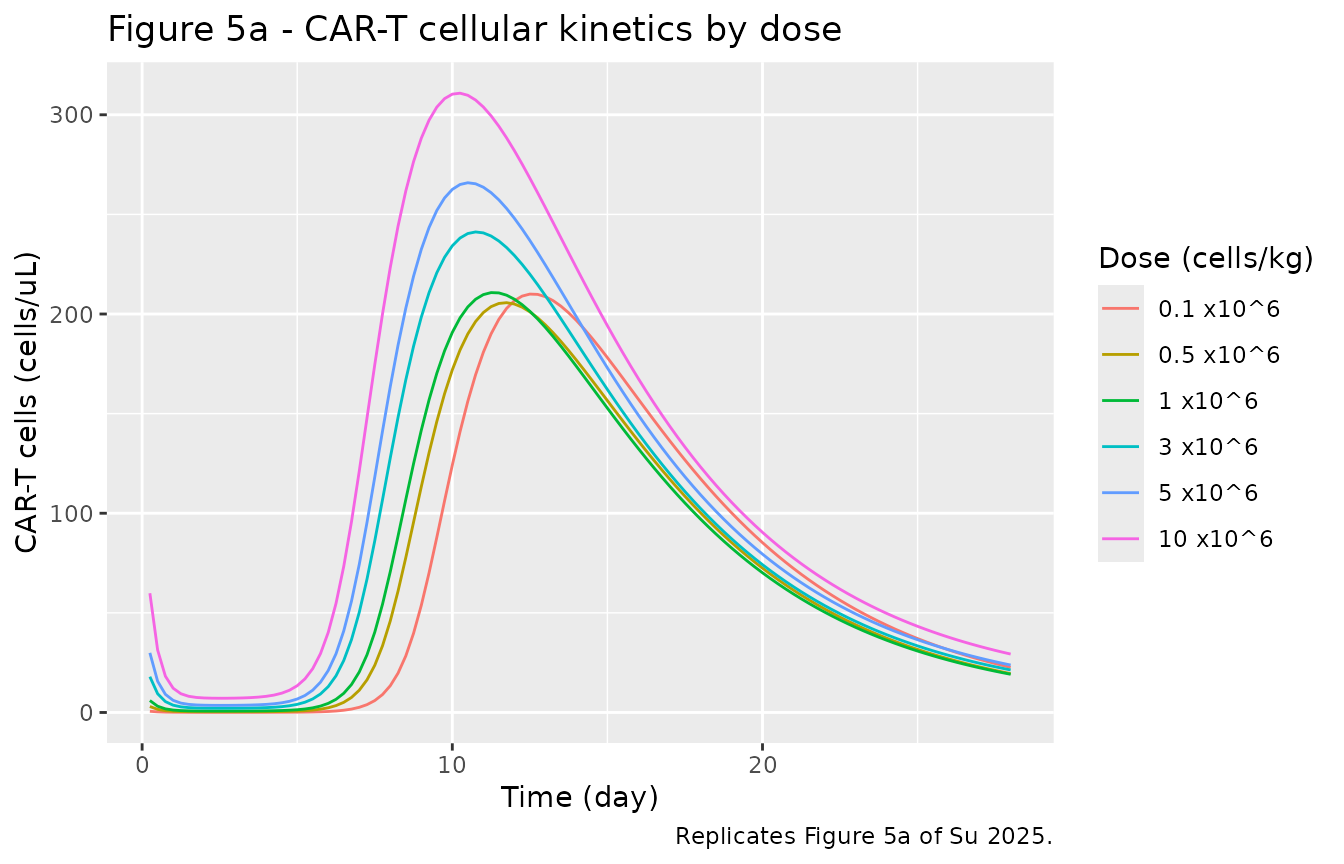
The model reproduces the four phases of CAR-T exposure (distribution,
expansion, contraction, persistence). We solve the typical-value model
(zeroRe) across the dose levels of Figure 5a. Because the
blood and bone-marrow volumes both scale with body weight and the dose
is per kg, body weight cancels from every output; the profiles below are
therefore age-invariant (the model’s AGE covariate is carried for
completeness).
mod_tv <- rxode2::zeroRe(mod_clin)
#> ℹ parameter labels from comments will be replaced by 'label()'

# Dose in CAR+ T cells/kg, split into memory/effector pools by the cohort-mean
# product composition (0.87:0.13). The model's f(cartm_pb)/f(carte_pb) = wt/Vb
# converts cells/kg to the blood concentration, so we dose the per-kg numbers.
dose_levels <- c(0.1, 0.5, 1, 3, 5, 10) * 1e6
mem_frac <- 0.87
eff_frac <- 0.13

solve_dose <- function(d, tmax = 28, dt = 0.25, age = 10) {
  ev <- rxode2::et(amt = d * mem_frac, cmt = "cartm_pb")
  ev <- rxode2::et(ev, amt = d * eff_frac, cmt = "carte_pb")
  # Observation rows sit on the blood effector state with dvid = 1 (the
  # `cells` endpoint); rxode2 returns both the `cells` and `transgene` outputs
  # as columns from a multi-endpoint model.
  ev <- rxode2::et(ev, seq(0, tmax, by = dt), cmt = "carte_pb") |> as.data.frame()
  ev$dvid <- ifelse(ev$evid == 0, 1L, NA_integer_)
  s <- as.data.frame(rxode2::rxSolve(mod_tv, ev, params = c(AGE = age), method = "lsoda", atol = 1e-9, rtol = 1e-9))
  s$dose <- d
  s
}

sim_tv <- dplyr::bind_rows(lapply(dose_levels, solve_dose))
#> ℹ omega/sigma items treated as zero: 'etalkmax_exp', 'etalkel_m', 'etalk12', 'etalkmax_kill'
#> ℹ omega/sigma items treated as zero: 'etalkmax_exp', 'etalkel_m', 'etalk12', 'etalkmax_kill'
#> ℹ omega/sigma items treated as zero: 'etalkmax_exp', 'etalkel_m', 'etalk12', 'etalkmax_kill'
#> ℹ omega/sigma items treated as zero: 'etalkmax_exp', 'etalkel_m', 'etalk12', 'etalkmax_kill'
#> ℹ omega/sigma items treated as zero: 'etalkmax_exp', 'etalkel_m', 'etalk12', 'etalkmax_kill'
#> ℹ omega/sigma items treated as zero: 'etalkmax_exp', 'etalkel_m', 'etalk12', 'etalkmax_kill'
sim_tv$dose_lbl <- factor(paste0(sim_tv$dose / 1e6, " x10^6"),
  levels = paste0(dose_levels / 1e6, " x10^6")
)
# Replicates Figure 5a of Su 2025: CAR-T cell concentration in peripheral blood
# across dose levels.
sim_tv |>
  dplyr::filter(time > 0) |>
  ggplot(aes(time, cells, colour = dose_lbl)) +
  geom_line() +
  labs(
    x = "Time (day)", y = "CAR-T cells (cells/uL)",
    colour = "Dose (cells/kg)",
    title = "Figure 5a - CAR-T cellular kinetics by dose",
    caption = "Replicates Figure 5a of Su 2025."
  )
Clinical CK-PD model: exposure vs. Table S3
Table S3 reports the simulated Cmax, Tmax and AUC0-28 of the CAR-T cell-count and qPCR-transgene profiles across dose levels. We reproduce those exposure metrics with PKNCA and compare them to the published values. The agreement is a direct check that the structural model and all fixed and estimated parameters were transcribed correctly.
# Fine grid to resolve Cmax/Tmax; 0-28 day window for AUC0-28.
sim_s3 <- dplyr::bind_rows(lapply(dose_levels, solve_dose, tmax = 28, dt = 0.1))
#> ℹ omega/sigma items treated as zero: 'etalkmax_exp', 'etalkel_m', 'etalk12', 'etalkmax_kill'
#> ℹ omega/sigma items treated as zero: 'etalkmax_exp', 'etalkel_m', 'etalk12', 'etalkmax_kill'
#> ℹ omega/sigma items treated as zero: 'etalkmax_exp', 'etalkel_m', 'etalk12', 'etalkmax_kill'
#> ℹ omega/sigma items treated as zero: 'etalkmax_exp', 'etalkel_m', 'etalk12', 'etalkmax_kill'
#> ℹ omega/sigma items treated as zero: 'etalkmax_exp', 'etalkel_m', 'etalk12', 'etalkmax_kill'
#> ℹ omega/sigma items treated as zero: 'etalkmax_exp', 'etalkel_m', 'etalk12', 'etalkmax_kill'
sim_s3$dose_lbl <- paste0(sim_s3$dose / 1e6, " x10^6")

# --- CAR-T cell-count output ---
conc_cells <- sim_s3 |>
  dplyr::filter(!is.na(cells)) |>
  dplyr::transmute(id = dose / 1e5, time, conc = cells, dose_lbl)
conc_cells <- dplyr::bind_rows(
  conc_cells,
  conc_cells |> dplyr::distinct(id, dose_lbl) |> dplyr::mutate(time = 0, conc = 0)
) |>
  dplyr::distinct(id, time, .keep_all = TRUE) |>
  dplyr::arrange(id, time)

ivals <- data.frame(start = 0, end = 28, cmax = TRUE, tmax = TRUE, auclast = TRUE)
nca_cells <- PKNCA::pk.nca(PKNCA::PKNCAdata(
  PKNCA::PKNCAconc(conc_cells, conc ~ time | dose_lbl + id),
  intervals = ivals
))
#> No dose information provided, calculations requiring dose will return NA.

# --- qPCR transgene output ---
conc_tg <- sim_s3 |>
  dplyr::filter(!is.na(transgene)) |>
  dplyr::transmute(id = dose / 1e5, time, conc = transgene, dose_lbl)
nca_tg <- PKNCA::pk.nca(PKNCA::PKNCAdata(
  PKNCA::PKNCAconc(conc_tg, conc ~ time | dose_lbl + id),
  intervals = data.frame(start = 0, end = 28, cmax = TRUE, tmax = TRUE, auclast = TRUE)
))
#> No dose information provided, calculations requiring dose will return NA.

summ <- function(nca) {
  as.data.frame(nca$result) |>
    dplyr::select(dose_lbl, PPTESTCD, PPORRES) |>
    tidyr::pivot_wider(names_from = PPTESTCD, values_from = PPORRES)
}
sim_cells <- summ(nca_cells)
sim_tg <- summ(nca_tg)
published <- tibble::tribble(
  ~dose_lbl, ~cmax_cell, ~tmax_cell, ~auc_cell, ~cmax_tg, ~tmax_tg, ~auc_tg,
  "0.1 x10^6", 202, 13, 2025, 152823, 13, 1271239,
  "0.5 x10^6", 208, 12, 2116, 159107, 12, 1335184,
  "1 x10^6", 210, 11, 2151, 160755, 11, 1356919,
  "3 x10^6", 242, 11, 2525, 197008, 11, 1677898,
  "5 x10^6", 266, 11, 2826, 224292, 11, 1949652,
  "10 x10^6", 313, 10, 3393, 282504, 10, 2488055
)

cmp <- published |>
  dplyr::left_join(
    sim_cells |> dplyr::transmute(dose_lbl, sim_cmax_cell = cmax, sim_tmax_cell = tmax, sim_auc_cell = auclast),
    by = "dose_lbl"
  ) |>
  dplyr::left_join(
    sim_tg |> dplyr::transmute(dose_lbl, sim_cmax_tg = cmax, sim_auc_tg = auclast),
    by = "dose_lbl"
  ) |>
  dplyr::mutate(
    `Cmax cell %diff` = round(100 * (sim_cmax_cell - cmax_cell) / cmax_cell, 1),
    `AUC cell %diff` = round(100 * (sim_auc_cell - auc_cell) / auc_cell, 1),
    `Cmax transgene %diff` = round(100 * (sim_cmax_tg - cmax_tg) / cmax_tg, 1),
    `AUC transgene %diff` = round(100 * (sim_auc_tg - auc_tg) / auc_tg, 1)
  )

cmp |>
  dplyr::transmute(
    Dose = dose_lbl,
    `Cmax cell (pub)` = cmax_cell, `Cmax cell (sim)` = round(sim_cmax_cell),
    `Tmax cell (pub)` = tmax_cell, `Tmax cell (sim)` = round(sim_tmax_cell),
    `AUC0-28 cell (pub)` = auc_cell, `AUC0-28 cell (sim)` = round(sim_auc_cell),
    `Cmax cell %diff`, `AUC cell %diff`
  ) |>
knitr::kable(caption = "Table S3a (cell-count): simulated vs. published CAR-T exposure.")| Dose | Cmax cell (pub) | Cmax cell (sim) | Tmax cell (pub) | Tmax cell (sim) | AUC0-28 cell (pub) | AUC0-28 cell (sim) | Cmax cell %diff | AUC cell %diff |
|---|---|---|---|---|---|---|---|---|
| 0.1 x10^6 | 202 | 210 | 13 | 13 | 2025 | 2099 | 4.0 | 3.6 |
| 0.5 x10^6 | 208 | 206 | 12 | 12 | 2116 | 2080 | -1.1 | -1.7 |
| 1 x10^6 | 210 | 211 | 11 | 11 | 2151 | 2147 | 0.4 | -0.2 |
| 3 x10^6 | 242 | 241 | 11 | 11 | 2525 | 2499 | -0.3 | -1.0 |
| 5 x10^6 | 266 | 266 | 11 | 10 | 2826 | 2788 | 0.0 | -1.3 |
| 10 x10^6 | 313 | 311 | 10 | 10 | 3393 | 3335 | -0.7 | -1.7 |
cmp |>
  dplyr::transmute(
    Dose = dose_lbl,
    `Cmax tg (pub)` = cmax_tg, `Cmax tg (sim)` = round(sim_cmax_tg),
    `AUC0-28 tg (pub)` = auc_tg, `AUC0-28 tg (sim)` = round(sim_auc_tg),
    `Cmax transgene %diff`, `AUC transgene %diff`
  ) |>
knitr::kable(caption = "Table S3a (transgene): simulated vs. published CAR-T exposure.")| Dose | Cmax tg (pub) | Cmax tg (sim) | AUC0-28 tg (pub) | AUC0-28 tg (sim) | Cmax transgene %diff | AUC transgene %diff |
|---|---|---|---|---|---|---|
| 0.1 x10^6 | 152823 | 161116 | 1271239 | 1335374 | 5.4 | 5.0 |
| 0.5 x10^6 | 159107 | 156406 | 1335184 | 1304454 | -1.7 | -2.3 |
| 1 x10^6 | 160755 | 161909 | 1356919 | 1355912 | 0.7 | -0.1 |
| 3 x10^6 | 197008 | 195770 | 1677898 | 1657502 | -0.6 | -1.2 |
| 5 x10^6 | 224292 | 224610 | 1949652 | 1918247 | 0.1 | -1.6 |
| 10 x10^6 | 282504 | 279992 | 2488055 | 2434884 | -0.9 | -2.1 |
# Structural check: the reproduced exposure metrics track the published values.
# A mis-transcribed rate constant, dose split or unit conversion would move
# these by tens of percent. The comparison is a deterministic typical-value
# reproduction (same parameters both sides), so the centre is tight; the
# loosest single point is the lowest-dose transgene Cmax, where the fixed
# log-log regression slope (1.41) amplifies the ~4% cell-level offset.
all_diffs <- c(
  cmp$`Cmax cell %diff`, cmp$`AUC cell %diff`,
  cmp$`Cmax transgene %diff`, cmp$`AUC transgene %diff`
)
stopifnot(
  abs(median(all_diffs)) < 3, # centre: structural fidelity
  max(abs(all_diffs)) < 8 # envelope across all dose levels and both outputs
)
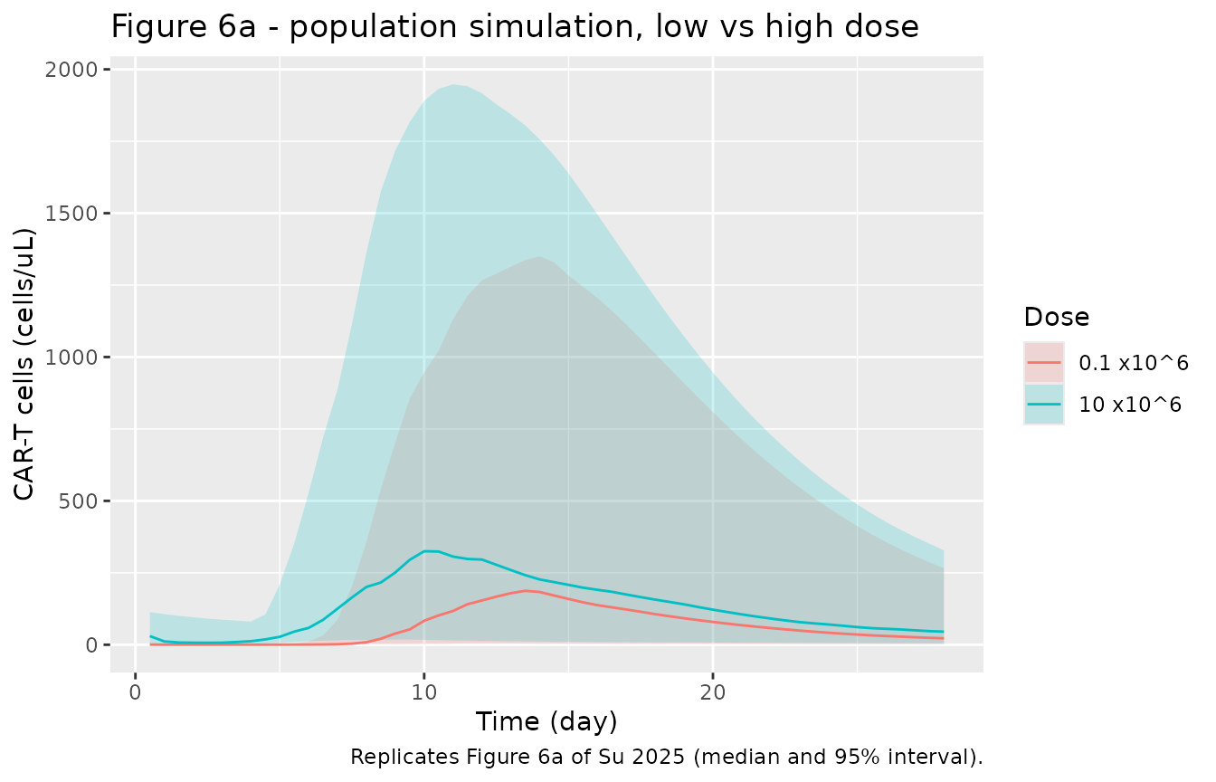
Clinical CK-PD model: population variability (Figure 6a)
The population simulation of Figure 6a overlays the low and high dose levels with between-subject variability on the expansion, elimination, distribution and killing rate constants. We draw a cohort of 100 subjects per dose arm (well within the 200/arm guideline).
set.seed(1234)
n_arm <- 100
pop_dose <- function(d, id_offset) {
  ev <- rxode2::et(amt = d * mem_frac, cmt = "cartm_pb")
  ev <- rxode2::et(ev, amt = d * eff_frac, cmt = "carte_pb")
  ev <- rxode2::et(ev, seq(0, 28, by = 0.5), cmt = "carte_pb") |> as.data.frame()
  ev$dvid <- ifelse(ev$evid == 0, 1L, NA_integer_)
  s <- as.data.frame(rxode2::rxSolve(mod_clin, ev, params = c(AGE = 10),
    nSub = n_arm, method = "lsoda", atol = 1e-8, rtol = 1e-8
  ))
  s$id <- s$sim.id + id_offset
  s$dose_lbl <- paste0(d / 1e6, " x10^6")
  s
}
sim_pop <- dplyr::bind_rows(
  pop_dose(0.1e6, 0L),
  pop_dose(10e6, 1000L)
)
#> ℹ parameter labels from comments will be replaced by 'label()'

sim_pop |>
  dplyr::filter(time > 0) |>
  dplyr::group_by(dose_lbl, time) |>
  dplyr::summarise(
    med = median(cells), lo = quantile(cells, 0.025), hi = quantile(cells, 0.975),
    .groups = "drop"
  ) |>
  ggplot(aes(time, med, colour = dose_lbl, fill = dose_lbl)) +
  geom_ribbon(aes(ymin = lo, ymax = hi), alpha = 0.2, colour = NA) +
  geom_line() +
  labs(
    x = "Time (day)", y = "CAR-T cells (cells/uL)", colour = "Dose", fill = "Dose",
    title = "Figure 6a - population simulation, low vs high dose",
    caption = "Replicates Figure 6a of Su 2025 (median and 95% interval)."
  )
In-vitro cell-level killing: B-ALL (Figure 2)
The in-vitro model seeds tumour and CAR T cells into a culture well and reads tumour-cell viability relative to the non-transduced control. We reproduce the RajiWT panel of Figure 2d: non-transduced T cells (NT), the single-targeted CD19 CAR (FMC63) and the dual-targeted AUTO3. The non-targeting CAR is represented by a near-zero association rate with the dissociation constant set high, exactly as the authors parameterised the control arms.
mod_ball <- rxode2::zeroRe(mod_vitro_ball)
#> ℹ parameter labels from comments will be replaced by 'label()'

solve_vitro <- function(mod, dens = list(), et_ratio = 1, tumor0 = 1e5, tmax = 3) {
  ev <- rxode2::et(amt = tumor0, cmt = "n_tumor")
  ev <- rxode2::et(ev, amt = et_ratio * tumor0, cmt = "n_cart")
  ev <- rxode2::et(ev, seq(0, tmax, by = 0.05))
  as.data.frame(rxode2::rxSolve(mod, ev, params = unlist(dens), method = "lsoda", atol = 1e-9, rtol = 1e-9))
}

raji <- list(dens_cd19_tumor = 50347, dens_cd22_tumor = 55116)
treatments <- list(
  NT = c(raji, list(kon_orig_cd19 = 1e-10, kon_orig_cd22 = 1e-10, kd_cd19 = 1e10, kd_cd22 = 1e10)),
  `CD19 CAR (FMC63)` = c(raji, list(kon_orig_cd19 = 207622, kon_orig_cd22 = 1e-10, kd_cd19 = 0.328, kd_cd22 = 1e10)),
  `CD19/CD22 CAR (AUTO3)` = raji
)

sim_ball <- dplyr::bind_rows(lapply(names(treatments), function(tx) {
  s <- solve_vitro(mod_ball, dens = treatments[[tx]])
  s$treatment <- tx
  s
}))
#> ℹ omega/sigma items treated as zero: 'etalkmax_kill', 'etalkc50_kill'
#> ℹ omega/sigma items treated as zero: 'etalkmax_kill', 'etalkc50_kill'
#> ℹ omega/sigma items treated as zero: 'etalkmax_kill', 'etalkc50_kill'
sim_ball$treatment <- factor(sim_ball$treatment, levels = names(treatments))

sim_ball |>
  ggplot(aes(time, viability, colour = treatment)) +
  geom_line() +
  labs(
    x = "Time (day)", y = "Tumour viability (% of control)", colour = "Treatment",
    title = "Figure 2d - RajiWT killing by CAR-T treatment",
    caption = "Replicates Figure 2d of Su 2025 (RajiWT, 1:1 ET ratio)."
  )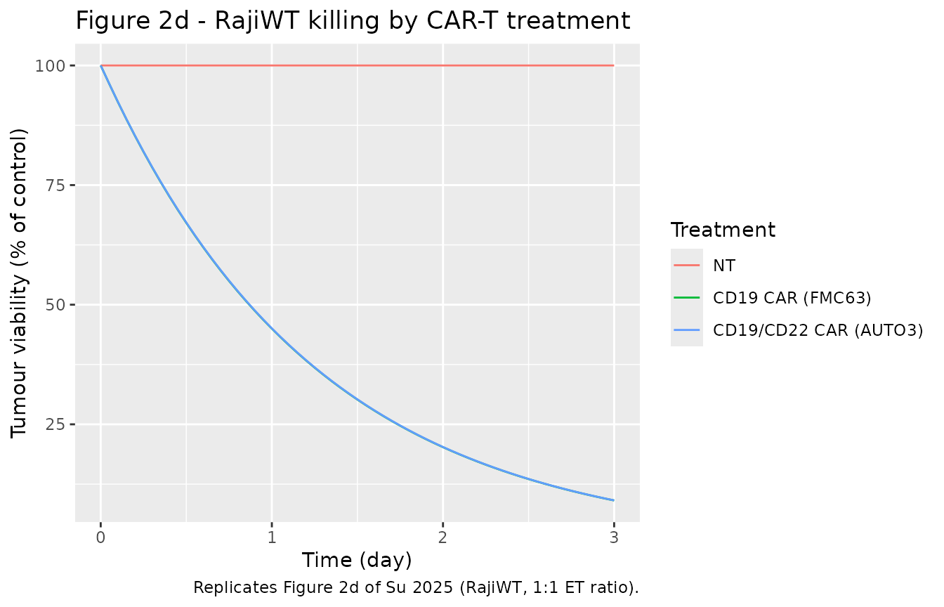
# Non-transduced control does not kill; the CAR-T arms do (RajiWT bears both
# antigens, so single-CD19 and dual AUTO3 both clear the line).
v24 <- sapply(names(treatments), function(tx) {
  s <- solve_vitro(mod_ball, dens = treatments[[tx]], tmax = 1)
  s$viability[nrow(s)]
})
#> ℹ omega/sigma items treated as zero: 'etalkmax_kill', 'etalkc50_kill'
#> ℹ omega/sigma items treated as zero: 'etalkmax_kill', 'etalkc50_kill'
#> ℹ omega/sigma items treated as zero: 'etalkmax_kill', 'etalkc50_kill'
stopifnot(v24[["NT"]] > 95, v24[["CD19/CD22 CAR (AUTO3)"]] < 70)
In-vitro cell-level killing: GPRC5D/BCMA, two co-stimulatory designs (Figure 3)
The independent multiple-myeloma dataset compares two bicistronic GPRC5D/BCMA constructs with distinct co-stimulatory domains. The CD28/41BB design (GCB4) estimated a superior potency (KC50 = 2.38 complexes/tumour cell) over the matched-41BB design (KC50 = 11.8), while the matched-41BB design has the higher maximum killing rate (KMaxKill = 4.39 vs. 2.71). We reproduce the cytotoxicity-vs-effector:target curves (Figure 3) on three cell lines and overlay the digitised observed means.
cell_dens <- list(
  RPMI8226 = list(dens_bcma_tumor = 12590, dens_gprc5d_tumor = 1184),
  OPM2WT = list(dens_bcma_tumor = 5000, dens_gprc5d_tumor = 746),
  MM1S = list(dens_bcma_tumor = 4300, dens_gprc5d_tumor = 746)
)
et_grid <- c(0, 0.03, 0.1, 0.3, 1)

mm_curve <- function(mod, label) {
  dplyr::bind_rows(lapply(names(cell_dens), function(cl) {
    dplyr::bind_rows(lapply(et_grid, function(et) {
      s <- solve_vitro(mod, dens = cell_dens[[cl]], et_ratio = et, tumor0 = 2e4, tmax = 1)
      data.frame(cell = cl, et = et, cytotox = 100 - s$viability[nrow(s)], construct = label)
    }))
  }))
}

mm <- dplyr::bind_rows(
  mm_curve(rxode2::zeroRe(mod_vitro_41bb), "GPRC5D-41BB-BCMA-41BB"),
  mm_curve(rxode2::zeroRe(mod_vitro_cd28), "GPRC5D-CD28-BCMA-41BB")
)
#> ℹ parameter labels from comments will be replaced by 'label()'
#> ℹ omega/sigma items treated as zero: 'etalkc50_kill'
#> ℹ omega/sigma items treated as zero: 'etalkc50_kill'
#> ℹ omega/sigma items treated as zero: 'etalkc50_kill'
#> ℹ omega/sigma items treated as zero: 'etalkc50_kill'
#> ℹ omega/sigma items treated as zero: 'etalkc50_kill'
#> ℹ omega/sigma items treated as zero: 'etalkc50_kill'
#> ℹ omega/sigma items treated as zero: 'etalkc50_kill'
#> ℹ omega/sigma items treated as zero: 'etalkc50_kill'
#> ℹ omega/sigma items treated as zero: 'etalkc50_kill'
#> ℹ omega/sigma items treated as zero: 'etalkc50_kill'
#> ℹ omega/sigma items treated as zero: 'etalkc50_kill'
#> ℹ omega/sigma items treated as zero: 'etalkc50_kill'
#> ℹ omega/sigma items treated as zero: 'etalkc50_kill'
#> ℹ omega/sigma items treated as zero: 'etalkc50_kill'
#> ℹ omega/sigma items treated as zero: 'etalkc50_kill'
#> ℹ parameter labels from comments will be replaced by 'label()'
#> ℹ omega/sigma items treated as zero: 'etalkmax_kill', 'etalkc50_kill'
#> ℹ omega/sigma items treated as zero: 'etalkmax_kill', 'etalkc50_kill'
#> ℹ omega/sigma items treated as zero: 'etalkmax_kill', 'etalkc50_kill'
#> ℹ omega/sigma items treated as zero: 'etalkmax_kill', 'etalkc50_kill'
#> ℹ omega/sigma items treated as zero: 'etalkmax_kill', 'etalkc50_kill'
#> ℹ omega/sigma items treated as zero: 'etalkmax_kill', 'etalkc50_kill'
#> ℹ omega/sigma items treated as zero: 'etalkmax_kill', 'etalkc50_kill'
#> ℹ omega/sigma items treated as zero: 'etalkmax_kill', 'etalkc50_kill'
#> ℹ omega/sigma items treated as zero: 'etalkmax_kill', 'etalkc50_kill'
#> ℹ omega/sigma items treated as zero: 'etalkmax_kill', 'etalkc50_kill'
#> ℹ omega/sigma items treated as zero: 'etalkmax_kill', 'etalkc50_kill'
#> ℹ omega/sigma items treated as zero: 'etalkmax_kill', 'etalkc50_kill'
#> ℹ omega/sigma items treated as zero: 'etalkmax_kill', 'etalkc50_kill'
#> ℹ omega/sigma items treated as zero: 'etalkmax_kill', 'etalkc50_kill'
#> ℹ omega/sigma items treated as zero: 'etalkmax_kill', 'etalkc50_kill'

# Digitised observed cytotoxicity means (Supplement 3 datasets).
mm_obs <- tibble::tribble(
  ~construct, ~cell, ~et, ~cytotox,
  "GPRC5D-41BB-BCMA-41BB", "RPMI8226", 0.03, 31.34, "GPRC5D-41BB-BCMA-41BB", "RPMI8226", 0.1, 70.03,
  "GPRC5D-41BB-BCMA-41BB", "RPMI8226", 0.3, 89.37, "GPRC5D-41BB-BCMA-41BB", "RPMI8226", 1, 98.91,
  "GPRC5D-41BB-BCMA-41BB", "OPM2WT", 0.03, 45.98, "GPRC5D-41BB-BCMA-41BB", "OPM2WT", 0.1, 54.02,
  "GPRC5D-41BB-BCMA-41BB", "OPM2WT", 0.3, 63.19, "GPRC5D-41BB-BCMA-41BB", "OPM2WT", 1, 79.69,
  "GPRC5D-41BB-BCMA-41BB", "MM1S", 0.03, 9.61, "GPRC5D-41BB-BCMA-41BB", "MM1S", 0.1, 22.20,
  "GPRC5D-41BB-BCMA-41BB", "MM1S", 0.3, 53.39, "GPRC5D-41BB-BCMA-41BB", "MM1S", 1, 87.87,
  "GPRC5D-CD28-BCMA-41BB", "RPMI8226", 0.03, 43.05, "GPRC5D-CD28-BCMA-41BB", "RPMI8226", 0.1, 49.86,
  "GPRC5D-CD28-BCMA-41BB", "RPMI8226", 0.3, 77.79, "GPRC5D-CD28-BCMA-41BB", "RPMI8226", 1, 92.23,
  "GPRC5D-CD28-BCMA-41BB", "OPM2WT", 0.03, 46.54, "GPRC5D-CD28-BCMA-41BB", "OPM2WT", 0.1, 59.10,
  "GPRC5D-CD28-BCMA-41BB", "OPM2WT", 0.3, 71.51, "GPRC5D-CD28-BCMA-41BB", "OPM2WT", 1, 88.29,
  "GPRC5D-CD28-BCMA-41BB", "MM1S", 0.03, 8.03, "GPRC5D-CD28-BCMA-41BB", "MM1S", 0.1, 32.76,
  "GPRC5D-CD28-BCMA-41BB", "MM1S", 0.3, 59.06, "GPRC5D-CD28-BCMA-41BB", "MM1S", 1, 93.23
)

ggplot(mm, aes(et, cytotox, colour = construct)) +
  geom_line() +
  geom_point(data = mm_obs, aes(et, cytotox, colour = construct), shape = 1, size = 2) +
  facet_wrap(~cell) +
  labs(
    x = "Effector : target ratio", y = "Cytotoxicity (% of control)",
    colour = "Construct",
    title = "Figure 3 - GPRC5D/BCMA cytotoxicity by co-stimulatory design",
    caption = "Lines: model; open points: digitised observed means. Replicates Figure 3 of Su 2025."
  )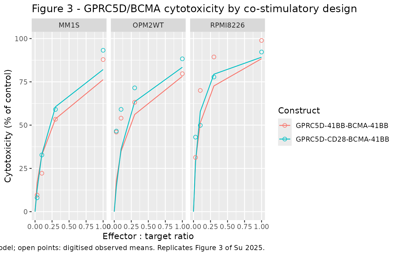
# Cytotoxicity rises monotonically with effector:target ratio for every
# construct x cell line (a structural property of the killing model).
mono <- mm |>
  dplyr::arrange(construct, cell, et) |>
  dplyr::group_by(construct, cell) |>
  dplyr::summarise(ok = all(diff(cytotox) > 0), .groups = "drop")
stopifnot(all(mono$ok))
Assumptions and deviations
-
Two outputs link by a fixed regression. The qPCR
transgene output is a fixed log-log function of the flow CAR-T cell
count (
ln(transgene) = 4.45 + 1.41 * ln(cells/uL)); both intercept and slope were fixed by the authors, so the two outputs carry the same information up to the transform. - Residual error recovered from the goodness-of-fit figures. Table 1 does not tabulate the residual-error magnitudes. The maintainers recovered them from the Monolix observations-vs-individual-predictions panels of Figure S2 by reading the 90% prediction-interval offsets: the qPCR output is proportional (SD = 0.73, from the censored-point band in Figure S2a/S2d), and the flow output is a combined additive-plus-proportional error (SD = 2.1 cells/uL + 0.54, from Figure S2b/S2f). These affect only the width of a simulated prediction interval, not the typical-value exposure predictions validated against Table S3.
-
Baseline antigen densities are encoded at the cohort
averages. The clinical model reads per-patient baseline CD19
(16666, range 1324-39098) and CD22 (4269, range 181-10137)
tumour-antigen densities as inputs. They are encoded here as fixed
parameters set to the cohort averages and are overridable per patient
(as in the Figure 5c antigen-density simulations), following the same
convention as the anti-BCMA CAR-T model
Su’s predecessorSingh_2021_idecabtageneVicleucel_human. -
Body weight cancels from the clinical outputs. The
blood and bone-marrow volumes both scale as
wt/70and the dose is per kg, so every reported output is independent of body weight (and hence of the AGE covariate). AGE is carried for fidelity to the published model structure. -
Printed-equation vs. as-run-code discrepancies resolved
toward the code. Several Supplement 1 display equations carry
transcription slips that the deposited Monolix code (Supplement 2)
corrects, and the model files follow the code: Eqs. 26/42 print the free
CD22 tumour antigen from the CD19 total (the code uses the CD22 total);
Eqs. 32-33/48-49 drop the
+before the double-target complex in the complex sum (the code adds all three); and Eqs. 48-49 divide the bone-marrow complex ratios by the blood CAR-T/tumour pools (the code divides by the bone-marrow pools). The clinical-model simulations reproduce Table S3 to within a few percent, confirming the code reading. -
In-vitro killing models carry no residual error.
Table 1 reports between- replicate variability on the in-vitro killing
potency but no residual-error magnitude, so the in-vitro observation
(
viability) is encoded with a fixed-zero additive error. The multiple-myeloma datasets report cytotoxicity (100 - viability); the models output viability and the figures above plot its complement. - As of the 2026-11 literature check there is no correction notice for this article. ```