Tacrolimus PK/PD in renal transplantation (Xiang 2025)
Source:vignettes/articles/Xiang_2025_tacrolimus.Rmd
Xiang_2025_tacrolimus.RmdModel and source
Xiang 2025 reports three models, extracted here as three model files that share this vignette:
pk   <- readModelDb("Xiang_2025_tacrolimus")
fpgm <- readModelDb("Xiang_2025_tacrolimus_fpg")
egfm <- readModelDb("Xiang_2025_tacrolimus_egfr")

ui_pk   <- rxode2::rxode(pk)
#> ℹ parameter labels from comments will be replaced by 'label()'
ui_fpg  <- rxode2::rxode(fpgm)
#> ℹ parameter labels from comments will be replaced by 'label()'
ui_egfr <- rxode2::rxode(egfm)
#> ℹ parameter labels from comments will be replaced by 'label()'- Citation: Xiang Q, Yang Y, Li G, Chen S, Yang Y, Liu L, Yu X. Population Pharmacokinetic/Pharmacodynamic Modeling of Tacrolimus in Renal Transplant Recipients: Impact of CYP3A5 Genotype and Wuzhi Capsule Co-Medication. Drug Des Devel Ther. 2025;19:8375-8389. doi:10.2147/DDDT.S542786. Parameter values are the final-model estimates in Table 2 (‘PPK model’ block); the structural equations are Eq. 1, 5 and 6.
- Article: https://doi.org/10.2147/DDDT.S542786
- Population PK: One-compartment population PK model with first-order absorption for oral tacrolimus in adult renal transplant recipients, built from twice-daily trough (C0) therapeutic drug monitoring data. Because no absorption-phase samples were collected the absorption rate constant is fixed at a literature value and the residual error is additive. Apparent clearance rises as a power function of post-operative day and is reduced by concomitant Wuzhi capsule and by the CYP3A53/3 non-expresser genotype; no covariate was retained on apparent volume of distribution. This is the population PK step of a three-model paper; the two sequential exposure-response models built on it are Xiang_2025_tacrolimus_fpg (fasting plasma glucose) and Xiang_2025_tacrolimus_egfr (estimated glomerular filtration rate).
- Exposure-response, fasting plasma glucose: Sequential exposure-response (PK/linear) model relating oral tacrolimus trough concentration to fasting plasma glucose in adult renal transplant recipients, as a quantitative model of post-transplantation diabetes mellitus risk. Fasting plasma glucose rises linearly from its pre-transplantation baseline with the predicted tacrolimus concentration; the baseline rises as a power function of age. The tacrolimus PK is the one-compartment model of the same paper, carried here as fixed parameters because the PK/PD model was fitted sequentially on the population PK step; see Xiang_2025_tacrolimus. The companion renal-function model in the same paper is Xiang_2025_tacrolimus_egfr.
- Exposure-response, eGFR: Sequential exposure-response (Imax) model relating oral tacrolimus trough concentration to the estimated glomerular filtration rate in adult renal transplant recipients, as a quantitative model of calcineurin-inhibitor nephrotoxicity. The eGFR falls from its post-transplant stable baseline by a saturable Imax function of the predicted tacrolimus concentration; the baseline falls with age and rises with hemoglobin. Both Imax and IC50 were fixed at clinically anchored values because they could not be estimated interpretably. The tacrolimus PK is the one-compartment model of the same paper, carried here as fixed parameters because the PK/PD model was fitted sequentially on the population PK step; see Xiang_2025_tacrolimus. The companion glucose model in the same paper is Xiang_2025_tacrolimus_fpg.
The paper builds the two exposure-response models
sequentially on the population PK model, so each PK/PD
file carries the PK parameters as fixed() values. That is
why all three files exist rather than one: Table 2 of the paper reports
three separate parameter blocks (“PPK model”, “C0-FPG model”, “C0-eGFR
model”), and the two PD models were fitted independently of one
another.
Population
The models were built on a retrospective single-centre cohort of 126 adult renal transplant recipients treated at the Second Affiliated Hospital of Chongqing Medical University between September 2021 and March 2024 (NCT05872815), randomly split 4:1 into an index group (n = 100) used for model building and an external validation group (n = 26). All parameter values extracted here are the index-group fit.
Index-group demographics (Xiang 2025 Table 1): 64% male; median age 38 years (range 19-65); median weight 60 kg (31-99); 92% Han ethnicity; median post-operative day 34 (range 0-182). CYP3A5 genotype was 1/1 in 8%, 1/3 in 31%, and 3/3 in 61%; the first two groups were pooled as “CYP3A5*1” expressers. Co-medications: Wuzhi capsule 33%, amlodipine 73%, metoprolol 65%, omeprazole 99%. Median tacrolimus dose 2.5 mg per administration (0.5-5.5), given twice daily; median trough 6.4 ng/mL (1.2-28.2). The analysis used 2279 tacrolimus troughs, 2055 fasting plasma glucose values and 2334 eGFR values.
The same information is available programmatically via each model’s
population metadata
(e.g. rxode2::rxode(readModelDb("Xiang_2025_tacrolimus"))$population).
Source trace
Per-parameter origins are recorded as in-file comments beside each
ini() entry. Collected here for review. Equation numbers
are those printed in the article; note that the text extracted from this
PDF drops every display equation, so equations 1-8 below were read from
the rendered PDF pages.
| Equation / parameter | Value | Source location |
|---|---|---|
IIV form, P_i = tvP * exp(eta_i)
|
n/a | Equation 1, p. 8377 |
FPG = FPG0 + beta * Cp,t |
n/a | Equation 2, p. 8377 |
eGFR = eGFR0 - Imax * Cp,t / (IC50 + Cp,t) |
n/a | Equation 3, p. 8377 |
ReGFR = (eGFR0 - eGFR) / eGFR0 * 100% |
n/a | Equation 4, p. 8378 |
V/F = 2248 L |
2248 | Equation 5, p. 8378; Table 2 |
CL/F = 33.7 * (POD/34)^0.109 * e^(-0.211*WZ) * e^(-0.381*Genotype) * e^(etaCL) |
n/a | Equation 6, p. 8378; covariate codings printed directly below it |
FPG0 = 4.2 * (Age/38)^0.232 * e^(etaFPG0) |
n/a | Equation 7, p. 8380 |
eGFR0 = 52.3 * (Age/38)^-0.403 * (HB/111)^0.254 * e^(etaeGFR0) |
n/a | Equation 8, p. 8381 |
lka (Ka) |
3.09 1/h, fixed | Table 2, PPK block (“3.09 FIX”); Discussion confirms 3.09 |
lvc (V/F) |
2248 L | Table 2, PPK block, Final Model (RSE 10.4%) |
lcl (CL/F) |
33.7 L/h | Table 2, PPK block, Final Model (RSE 6.9%) |
e_pod_cl |
0.109 | Table 2, “POD on CL/F” (RSE 4.7%) |
e_conmed_wuzhi_cl |
-0.211 | Table 2, “WZ on CL/F” (RSE 8.5%) |
e_cyp3a5_expr_cl |
-0.381 | Table 2, “CYP3A53/3 on CL/F” (RSE 21.1%) |
etalcl |
32.6% CV | Table 2, “IIV CL/F (%)” (RSE 17.1%) |
etalvc |
88.6% CV | Table 2, “IIV V/F (%)” (RSE 19.3%) |
addSd (PK) |
2.20 ng/mL | Table 2, “Residual error Additive (ng/mL)” |
lrbase_fpg (FPG0) |
4.2 mmol/L | Table 2, C0-FPG block (RSE 2.3%) |
lslope (beta) |
0.264, fixed | Table 2, C0-FPG block (“0.264 FIX”); Discussion gives the provenance |
e_age_rbase_fpg |
0.232 | Table 2, “Age on FPG0” (RSE 23.9%) |
etalrbase_fpg |
17.0% CV | Table 2, “IIV FPG0 (%)” (RSE 19.9%) |
propSd (FPG) |
23.1% | Table 2, C0-FPG “Residual error Proportional (%)” |
lrbase_egfr (eGFR0) |
52.3 mL/min/1.73 m^2 | Table 2, C0-eGFR block (RSE 2.8%) |
limax (Imax) |
30 mL/min/1.73 m^2, fixed | Table 2, C0-eGFR block (“30 FIX”); Discussion gives the CKD-stage-4 anchor |
lic50 (IC50) |
10 ng/mL, fixed | Table 2, C0-eGFR block (“10 FIX”); Discussion gives the nephrotoxicity-incidence anchor |
e_age_rbase_egfr |
-0.403 | Table 2, “Age on eGFR0” (RSE 14.8%) |
e_hgb_rbase_egfr |
0.254 | Table 2, “HB on eGFR0” (RSE 4.9%) |
etalrbase_egfr |
22.1% CV | Table 2, “IIV eGFR0 (%)” (RSE 13.8%) |
propSd (eGFR) |
17.2% | Table 2, C0-eGFR “Residual error Proportional (%)” |
Virtual cohort
Original observed data are not publicly available (the paper’s Data Sharing Statement declines to share individual participant data). The simulations below use the four covariate subgroups the paper itself simulated, defined by the two binary covariates retained on CL/F.
Note the value inversion on genotype: the paper codes
Genotype = 1 for the CYP3A53/3 non-expresser,
while the canonical column CYP3A5_EXPR codes 1
for the expresser. The model applies the published coefficient to
(1 - CYP3A5_EXPR), so the four subgroups below map
one-to-one onto the paper’s.
subgroups <- tibble::tribble(
  ~subgroup,                 ~CYP3A5_EXPR, ~CONMED_WUZHI,
  "CYP3A5*1, no WZ",         1,            0,
  "CYP3A5*1, + WZ",          1,            1,
  "CYP3A5*3/*3, no WZ",      0,            0,
  "CYP3A5*3/*3, + WZ",       0,            1
)

# Typical covariate values: the index-cohort medians the model is centred on.
AGE_MEDIAN <- 38   # years    (Table 1)
HGB_MEDIAN <- 111  # g/L      (Table 1)

TAU        <- 12   # h, q12h dosing
DAYS       <- 30   # simulate one month, as the paper's Figure 4 does
POD_START  <- 1    # tacrolimus began within 24 h of transplantation
doses_mg   <- c(1, 2, 3, 4)

# CYP3A5 star-allele labels contain '*', which pandoc would otherwise consume as
# markdown emphasis ("CYP3A5*3/*3" renders as "CYP3A53/3"). Escape it for tables
# only; the unescaped form is what the plots and the grouping keys use.
md_escape <- function(x) gsub("*", "\\*", x, fixed = TRUE)

TDM_LOW  <- 6      # ng/mL, the paper's target trough range (Chinese guidance)
TDM_HIGH <- 10
FPG_PTDM <- 7.0    # mmol/L, the paper's PTDM threshold
REGFR_INJURY <- 20 # %, the paper's renal-impairment threshold
Event tables are built by a single helper so the PK, FPG and eGFR simulations all see an identical dosing and covariate history. Observations are placed just before each dose, i.e. at the trough, because the trough is the concentration the paper’s PK model was fitted to and the concentration its two PD equations take as their driver.
POD is time-varying: it advances one day per 24 h of
simulated time. Observation rows carry cmt = "central" (the
ODE state), never the name of an algebraic observable.
make_events <- function(subgroup, dose, n = 1L, id_offset = 0L,
                        pod_start = POD_START, days = DAYS,
                        age = AGE_MEDIAN, hgb = HGB_MEDIAN) {
  sg <- subgroups[subgroups$subgroup == subgroup, ]
  stopifnot(nrow(sg) == 1L)

  n_dose <- days * 24 / TAU
  dose_times <- seq(0, by = TAU, length.out = n_dose)
  # Troughs: 0.01 h before each dose after the first, plus the end of the month.
  obs_times <- c(dose_times[-1], n_dose * TAU) - 0.01

  subj <- tibble::tibble(id = id_offset + seq_len(n))

  dosing <- tidyr::crossing(subj, time = dose_times) |>
    dplyr::mutate(evid = 1L, amt = dose, cmt = "depot")
  obs <- tidyr::crossing(subj, time = obs_times) |>
    dplyr::mutate(evid = 0L, amt = NA_real_, cmt = "central")

  dplyr::bind_rows(dosing, obs) |>
    dplyr::arrange(id, time, dplyr::desc(evid)) |>
    dplyr::mutate(
      subgroup     = subgroup,
      dose_mg      = dose,
      regimen      = paste0(dose, " mg q12h"),
      arm          = paste0(subgroup, " | ", dose, " mg q12h"),
      CYP3A5_EXPR  = sg$CYP3A5_EXPR,
      CONMED_WUZHI = sg$CONMED_WUZHI,
      AGE          = age,
      HGB          = hgb,
      POD          = pod_start + time / 24
    )
}
Simulation
Typical-value profiles: the paper’s Figure 4 grid
Sixteen arms (four covariate subgroups x four dose levels), simulated with the random effects zeroed so each curve is the typical-value prediction the paper’s Figure 4 shows.
grid16 <- tidyr::crossing(subgroup = subgroups$subgroup, dose = doses_mg) |>
  dplyr::mutate(id_offset = seq_len(dplyr::n()) - 1L)

ev_typ <- do.call(
  dplyr::bind_rows,
  Map(make_events,
      subgroup  = grid16$subgroup,
      dose      = grid16$dose,
      id_offset = grid16$id_offset,
      MoreArgs  = list(n = 1L))
)
stopifnot(!anyDuplicated(unique(ev_typ[, c("id", "time", "evid")])))

keep_cols <- c("subgroup", "dose_mg", "regimen", "arm", "POD")

sim_pk_typ <- rxode2::rxSolve(
  rxode2::zeroRe(pk), events = as.data.frame(ev_typ), keep = keep_cols
) |> as.data.frame()
#> ℹ parameter labels from comments will be replaced by 'label()'
#> ℹ omega/sigma items treated as zero: 'etalcl', 'etalvc'
#> Warning: multi-subject simulation without without 'omega'

sim_fpg_typ <- rxode2::rxSolve(
  rxode2::zeroRe(fpgm), events = as.data.frame(ev_typ), keep = keep_cols
) |> as.data.frame()
#> ℹ parameter labels from comments will be replaced by 'label()'
#> ℹ omega/sigma items treated as zero: 'etalcl', 'etalvc', 'etalrbase_fpg'
#> Warning: multi-subject simulation without without 'omega'

if (is.null(sim_pk_typ$id))  sim_pk_typ$id  <- 1L
if (is.null(sim_fpg_typ$id)) sim_fpg_typ$id <- 1L

stopifnot(nrow(sim_pk_typ) > 0, !all(is.na(sim_pk_typ$Cc)))
stopifnot(nrow(sim_fpg_typ) > 0, !all(is.na(sim_fpg_typ$fpg)))
The eGFR model is simulated over the window the paper used for it:
one month beginning on post-operative day 7, the day the authors took
renal function to have stabilised and therefore the day
eGFR0 is anchored to.
ev_egfr <- do.call(
  dplyr::bind_rows,
  Map(make_events,
      subgroup  = grid16$subgroup,
      dose      = grid16$dose,
      id_offset = grid16$id_offset,
      MoreArgs  = list(n = 1L, pod_start = 7))
)
stopifnot(!anyDuplicated(unique(ev_egfr[, c("id", "time", "evid")])))

sim_egfr_typ <- rxode2::rxSolve(
  rxode2::zeroRe(egfm), events = as.data.frame(ev_egfr), keep = keep_cols
) |> as.data.frame()
#> ℹ parameter labels from comments will be replaced by 'label()'
#> ℹ omega/sigma items treated as zero: 'etalcl', 'etalvc', 'etalrbase_egfr'
#> Warning: multi-subject simulation without without 'omega'
if (is.null(sim_egfr_typ$id)) sim_egfr_typ$id <- 1L

# ReGFR, Equation 4. rbase_egfr is returned by rxSolve as a model variable.
sim_egfr_typ <- sim_egfr_typ |>
  dplyr::mutate(ReGFR = (rbase_egfr - egfr) / rbase_egfr * 100)

stopifnot(nrow(sim_egfr_typ) > 0, !all(is.na(sim_egfr_typ$ReGFR)))
Population profiles with between-subject variability
One hundred subjects per subgroup at the paper’s common maintenance dose of 2 mg q12h, carrying the model’s inter-individual variability.
set.seed(20250918)
N_PER_ARM <- 100L

ev_pop <- do.call(
  dplyr::bind_rows,
  Map(make_events,
      subgroup  = subgroups$subgroup,
      id_offset = (seq_len(nrow(subgroups)) - 1L) * N_PER_ARM,
      MoreArgs  = list(dose = 2, n = N_PER_ARM))
)
stopifnot(!anyDuplicated(unique(ev_pop[, c("id", "time", "evid")])))

sim_pop <- rxode2::rxSolve(pk, events = as.data.frame(ev_pop), keep = keep_cols) |>
  as.data.frame()
#> ℹ parameter labels from comments will be replaced by 'label()'

stopifnot(dplyr::n_distinct(sim_pop$id) == nrow(subgroups) * N_PER_ARM)
Replicate published figures
Figure 4a - tacrolimus trough by subgroup and dose
# Replicates Figure 4a of Xiang 2025: typical trough time course over the first
# post-operative month, four subgroups, 1-4 mg q12h. Dashed lines are the
# 6-10 ng/mL TDM target range.
sim_pk_typ |>
  ggplot(aes(POD, Cc, colour = regimen)) +
  geom_hline(yintercept = c(TDM_LOW, TDM_HIGH), linetype = "dashed") +
  geom_line() +
  facet_wrap(~subgroup) +
  labs(x = "Post-operative day", y = "Tacrolimus trough C0 (ng/mL)",
       colour = "Regimen",
       title = "Figure 4a - typical trough concentration",
       caption = "Replicates Figure 4a of Xiang 2025.")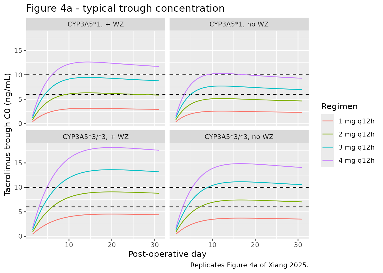
Troughs fall over the month at a constant dose because CL/F rises with post-operative day, exactly as the paper describes (“C0 decreased with time after transplantation in the simulations because the CL/F of tacrolimus increased with POD”).
Figure 4b - fasting plasma glucose by subgroup and dose
# Replicates Figure 4b of Xiang 2025. Dashed line is the 7.0 mmol/L PTDM
# threshold.
sim_fpg_typ |>
  ggplot(aes(POD, fpg, colour = regimen)) +
  geom_hline(yintercept = FPG_PTDM, linetype = "dashed") +
  geom_line() +
  facet_wrap(~subgroup) +
  labs(x = "Post-operative day", y = "Fasting plasma glucose (mmol/L)",
       colour = "Regimen",
       title = "Figure 4b - typical fasting plasma glucose",
       caption = "Replicates Figure 4b of Xiang 2025.")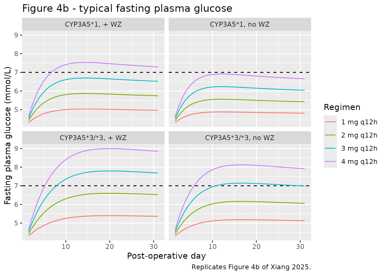
Supplementary Figure 3 - relative eGFR by subgroup and dose
# Replicates Supplementary Figure 3 of Xiang 2025: relative eGFR decline over
# one month starting post-operative day 7. Dashed line is the 20% renal-injury
# threshold.
sim_egfr_typ |>
  ggplot(aes(POD, ReGFR, colour = regimen)) +
  geom_hline(yintercept = REGFR_INJURY, linetype = "dashed") +
  geom_line() +
  facet_wrap(~subgroup) +
  labs(x = "Post-operative day", y = "Relative eGFR decline ReGFR (%)",
       colour = "Regimen",
       title = "Supplementary Figure 3 - typical relative eGFR decline",
       caption = "Replicates Supplementary Figure 3 of Xiang 2025.")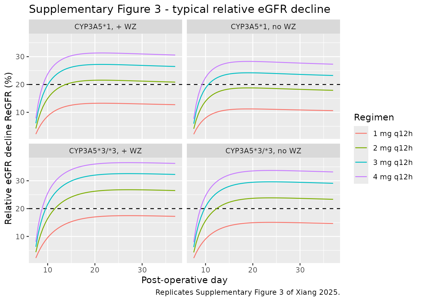
Between-subject variability at 2 mg q12h
sim_pop |>
  dplyr::group_by(subgroup, POD) |>
  dplyr::summarise(
    Q05 = quantile(Cc, 0.05, na.rm = TRUE),
    Q50 = quantile(Cc, 0.50, na.rm = TRUE),
    Q95 = quantile(Cc, 0.95, na.rm = TRUE),
    .groups = "drop"
  ) |>
  ggplot(aes(POD, Q50)) +
  geom_ribbon(aes(ymin = Q05, ymax = Q95), alpha = 0.25) +
  geom_hline(yintercept = c(TDM_LOW, TDM_HIGH), linetype = "dashed") +
  geom_line() +
  facet_wrap(~subgroup) +
  labs(x = "Post-operative day", y = "Tacrolimus trough C0 (ng/mL)",
       title = "Trough distribution at 2 mg q12h (median and 5th-95th percentile)",
       caption = "100 simulated subjects per subgroup.")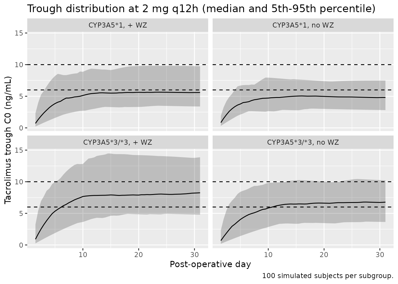
PKNCA validation
Xiang 2025 reports no non-compartmental analysis: the dataset is trough-only therapeutic drug monitoring, and the paper publishes no Cmax, Tmax, AUC or half-life table to compare against. The Discussion says so directly, and names it as a limitation (“the population PK model was established only from trough concentrations of tacrolimus and lacked the necessary information to estimate the absorption parameters”).
PKNCA is therefore used here for what it can establish: that
the packaged model is internally consistent at steady state, by checking
the exposure identity AUCtau = Dose / (CL/F) per subject.
This is a structural identity of a one-compartment model at steady
state, so it must hold to within numerical tolerance for every simulated
subject; if it does not, the unit conversion or the covariate model is
wrong.
This block deliberately departs from the figures above in two ways, so that the identity it checks is actually true and any deviation is attributable to the model rather than to the simulation design.
-
PODis frozen at the day-30 value.AUCtau = Dose / (CL/F)is a steady-state result, and the model’s clearance rises with post-operative day by construction, so under the time-varying covariate the system never quite reaches steady state - the drug still in the body was accumulated when clearance was lower, and the AUC sits about 1% aboveDose / (CL/F). That lag is a correct consequence of the published covariate model, not an error, but it would mask what this check is for. - The dosing history is longer than one month. The slowest-clearing subgroup (CYP3A53/3 on the Wuzhi capsule) has a terminal half-life near 84 h, so after 30 days it is still about 0.3% short of steady state. A 200-day history puts every arm fully at steady state.
A dense 0.1 h grid over the final dosing interval resolves Cmax and the distribution phase.
POD_NCA   <- POD_START + (DAYS * 24 - TAU) / 24  # day-30 value, held constant
N_DOSE_SS <- 400L                                # 200 days q12h; >50 half-lives
ss_start  <- (N_DOSE_SS - 1) * TAU

arms <- ev_typ |>
  dplyr::distinct(id, subgroup, dose_mg, regimen, arm,
                  CYP3A5_EXPR, CONMED_WUZHI, AGE, HGB)

ev_ss <- arms |>
  tidyr::crossing(time = seq(0, by = TAU, length.out = N_DOSE_SS)) |>
  dplyr::mutate(evid = 1L, cmt = "depot") |>
  dplyr::rename(amt = dose_mg) |>
  dplyr::mutate(dose_mg = amt)

dense_obs <- arms |>
  tidyr::crossing(toff = seq(0, TAU, by = 0.1)) |>
  dplyr::mutate(
    time = ss_start + toff,
    evid = 0L, amt = NA_real_, cmt = "central"
  ) |>
  dplyr::select(-toff)

ev_nca <- dplyr::bind_rows(ev_ss, dense_obs) |>
  dplyr::mutate(POD = POD_NCA) |>       # freeze POD: see note above
  dplyr::arrange(id, time, dplyr::desc(evid))

sim_nca_raw <- rxode2::rxSolve(
  rxode2::zeroRe(pk), events = as.data.frame(ev_nca),
  keep = c("subgroup", "dose_mg", "regimen", "arm")
) |> as.data.frame()
#> ℹ parameter labels from comments will be replaced by 'label()'
#> ℹ omega/sigma items treated as zero: 'etalcl', 'etalvc'
#> Warning: multi-subject simulation without without 'omega'
if (is.null(sim_nca_raw$id)) sim_nca_raw$id <- 1L
# Filter on !is.na(Cc) ONLY - adding time > 0 or Cc > 0 would drop the
# interval-anchoring first record and trigger PKNCA's AUC-range warning.
sim_nca <- sim_nca_raw |>
  dplyr::filter(!is.na(Cc)) |>
  dplyr::mutate(time = time - ss_start) |>   # re-base the interval at 0
  dplyr::select(id, time, Cc, arm)

stopifnot(nrow(sim_nca) > 0)

conc_obj <- PKNCA::PKNCAconc(sim_nca, Cc ~ time | arm + id)

dose_df <- ev_nca |>
  dplyr::filter(evid == 1, time == ss_start) |>
  dplyr::mutate(time = 0) |>
  dplyr::select(id, time, amt, arm)

dose_obj <- PKNCA::PKNCAdose(dose_df, amt ~ time | arm + id)

intervals <- data.frame(
  start   = 0,
  end     = TAU,
  cmax    = TRUE,
  tmax    = TRUE,
  cmin    = TRUE,
  auclast = TRUE
)

nca_res <- PKNCA::pk.nca(PKNCA::PKNCAdata(conc_obj, dose_obj, intervals = intervals))
nca_wide <- as.data.frame(nca_res) |>
  dplyr::select(arm, id, PPTESTCD, PPORRES) |>
  tidyr::pivot_wider(names_from = PPTESTCD, values_from = PPORRES)

stopifnot(nrow(nca_wide) == nrow(grid16))
Structural identity: AUCtau = Dose / (CL/F)
cl_by_id <- sim_nca_raw |>
  dplyr::group_by(id, arm, dose_mg) |>
  dplyr::summarise(cl = mean(cl), .groups = "drop")

identity_tbl <- nca_wide |>
  dplyr::left_join(cl_by_id, by = c("id", "arm")) |>
  dplyr::mutate(
    # auclast is in ng/mL * h; Dose/CL in mg / (L/h) = mg*h/L = 1000 ng*h/mL
    auc_expected = dose_mg / cl * 1000,
    pct_diff     = (auclast - auc_expected) / auc_expected * 100
  )

stopifnot(nrow(identity_tbl) == nrow(grid16), !anyNA(identity_tbl$pct_diff))

# With POD frozen the system is at true steady state, so the only gap between
# the trapezoidal AUC and Dose/CL is grid discretisation.
stopifnot(max(abs(identity_tbl$pct_diff)) < 0.05)

identity_tbl |>
  dplyr::select(arm, auclast, auc_expected, pct_diff) |>
  dplyr::arrange(arm) |>
  dplyr::mutate(arm = md_escape(arm)) |>
  dplyr::rename(
    "Subgroup | regimen"           = arm,
    "AUCtau, PKNCA (ng*h/mL)"      = auclast,
    "Dose / (CL/F) (ng*h/mL)"      = auc_expected,
    "Difference (%)"               = pct_diff
  ) |>
  knitr::kable(
    digits  = c(0, 1, 1, 3),
    caption = "Steady-state exposure identity check, all 16 typical-value arms."
)| Subgroup | regimen | AUCtau, PKNCA (ng*h/mL) | Dose / (CL/F) (ng*h/mL) | Difference (%) |
|---|---|---|---|
| CYP3A5*1, + WZ | 1 mg q12h | 37.1 | 37.1 | -0.003 |
| CYP3A5*1, + WZ | 2 mg q12h | 74.2 | 74.2 | -0.003 |
| CYP3A5*1, + WZ | 3 mg q12h | 111.2 | 111.2 | -0.003 |
| CYP3A5*1, + WZ | 4 mg q12h | 148.3 | 148.3 | -0.003 |
| CYP3A5*1, no WZ | 1 mg q12h | 30.0 | 30.0 | -0.004 |
| CYP3A5*1, no WZ | 2 mg q12h | 60.1 | 60.1 | -0.004 |
| CYP3A5*1, no WZ | 3 mg q12h | 90.1 | 90.1 | -0.004 |
| CYP3A5*1, no WZ | 4 mg q12h | 120.1 | 120.1 | -0.004 |
| CYP3A5*3/*3, + WZ | 1 mg q12h | 54.3 | 54.3 | -0.002 |
| CYP3A5*3/*3, + WZ | 2 mg q12h | 108.6 | 108.6 | -0.002 |
| CYP3A5*3/*3, + WZ | 3 mg q12h | 162.8 | 162.8 | -0.002 |
| CYP3A5*3/*3, + WZ | 4 mg q12h | 217.1 | 217.1 | -0.002 |
| CYP3A5*3/*3, no WZ | 1 mg q12h | 44.0 | 44.0 | -0.003 |
| CYP3A5*3/*3, no WZ | 2 mg q12h | 87.9 | 87.9 | -0.003 |
| CYP3A5*3/*3, no WZ | 3 mg q12h | 131.9 | 131.9 | -0.003 |
| CYP3A5*3/*3, no WZ | 4 mg q12h | 175.8 | 175.8 | -0.003 |
The largest deviation is 0.004%, which is the trapezoidal-rule discretisation error on a 0.1 h grid. The unit conversion (1 mg/L = 1000 ng/mL) and the covariate model are therefore consistent.
Steady-state summary by subgroup and dose
nca_wide |>
  dplyr::arrange(arm) |>
  dplyr::select(arm, cmax, tmax, cmin, auclast) |>
  dplyr::mutate(arm = md_escape(arm)) |>
  dplyr::rename(
    "Subgroup | regimen"     = arm,
    "Cmax (ng/mL)"           = cmax,
    "Tmax (h)"               = tmax,
    "Cmin (ng/mL)"           = cmin,
    "AUCtau (ng*h/mL)"       = auclast
  ) |>
  knitr::kable(
    digits  = c(0, 2, 2, 2, 1),
    caption = "Simulated steady-state NCA over one 12 h interval (typical values). Xiang 2025 publishes no NCA table to compare against; these values are reported so the model's exposure metrics are inspectable."
)| Subgroup | regimen | Cmax (ng/mL) | Tmax (h) | Cmin (ng/mL) | AUCtau (ng*h/mL) |
|---|---|---|---|---|
| CYP3A5*1, + WZ | 1 mg q12h | 3.27 | 1.2 | 2.88 | 37.1 |
| CYP3A5*1, + WZ | 2 mg q12h | 6.54 | 1.2 | 5.77 | 74.2 |
| CYP3A5*1, + WZ | 3 mg q12h | 9.82 | 1.2 | 8.65 | 111.2 |
| CYP3A5*1, + WZ | 4 mg q12h | 13.09 | 1.2 | 11.54 | 148.3 |
| CYP3A5*1, no WZ | 1 mg q12h | 2.69 | 1.1 | 2.30 | 30.0 |
| CYP3A5*1, no WZ | 2 mg q12h | 5.37 | 1.1 | 4.59 | 60.1 |
| CYP3A5*1, no WZ | 3 mg q12h | 8.06 | 1.1 | 6.89 | 90.1 |
| CYP3A5*1, no WZ | 4 mg q12h | 10.74 | 1.1 | 9.19 | 120.1 |
| CYP3A5*3/*3, + WZ | 1 mg q12h | 4.70 | 1.2 | 4.32 | 54.3 |
| CYP3A5*3/*3, + WZ | 2 mg q12h | 9.41 | 1.2 | 8.63 | 108.6 |
| CYP3A5*3/*3, + WZ | 3 mg q12h | 14.11 | 1.2 | 12.95 | 162.8 |
| CYP3A5*3/*3, + WZ | 4 mg q12h | 18.82 | 1.2 | 17.26 | 217.1 |
| CYP3A5*3/*3, no WZ | 1 mg q12h | 3.84 | 1.2 | 3.46 | 44.0 |
| CYP3A5*3/*3, no WZ | 2 mg q12h | 7.69 | 1.2 | 6.91 | 87.9 |
| CYP3A5*3/*3, no WZ | 3 mg q12h | 11.53 | 1.2 | 10.37 | 131.9 |
| CYP3A5*3/*3, no WZ | 4 mg q12h | 15.38 | 1.2 | 13.82 | 175.8 |
The profile is nearly flat within the dosing interval (46.2 h terminal half-life at the reference covariates against a 12 h interval), which is why trough-only sampling is enough to identify CL/F and why the trough is a good surrogate for average exposure in this model.
Comparison against the paper’s quantitative claims
In place of an NCA comparison, the model is scored against the six numeric claims Xiang 2025 makes from its own simulations. Each is evaluated on the typical-value predictions above.
# Trough on the last simulated day of the month, per arm, from the Figure 4a
# simulation; and the corresponding FPG and ReGFR.
last_pk <- sim_pk_typ |>
  dplyr::group_by(arm, subgroup, dose_mg) |>
  dplyr::slice_max(time, n = 1) |>
  dplyr::ungroup() |>
  dplyr::select(subgroup, dose_mg, C0_last = Cc)

# Day 7 is the paper's decision point for "reaching the TDM range within
# 7 days of administration".
day7_pk <- sim_pk_typ |>
  dplyr::filter(POD <= 8) |>
  dplyr::group_by(subgroup, dose_mg) |>
  dplyr::slice_max(time, n = 1) |>
  dplyr::ungroup() |>
  dplyr::select(subgroup, dose_mg, C0_day7 = Cc)

fpg_max <- sim_fpg_typ |>
  dplyr::group_by(subgroup, dose_mg) |>
  dplyr::summarise(FPG_max = max(fpg), .groups = "drop")

regfr_max <- sim_egfr_typ |>
  dplyr::group_by(subgroup, dose_mg) |>
  dplyr::summarise(ReGFR_max = max(ReGFR), .groups = "drop")

claims_data <- day7_pk |>
  dplyr::left_join(last_pk,   by = c("subgroup", "dose_mg")) |>
  dplyr::left_join(fpg_max,   by = c("subgroup", "dose_mg")) |>
  dplyr::left_join(regfr_max, by = c("subgroup", "dose_mg"))

stopifnot(nrow(claims_data) == nrow(grid16), !anyNA(claims_data$C0_day7))

# Fail loudly rather than silently returning a zero-row TRUE (a lookup that
# matches nothing would make all() vacuously true).
cell <- function(sg, d, col) {
  v <- claims_data[[col]][claims_data$subgroup == sg & claims_data$dose_mg == d]
  if (length(v) != 1L) stop("no unique row for '", sg, "' at ", d, " mg")
  v
}

claims <- tibble::tribble(
  ~claim, ~quantity, ~value, ~passes,

  "CYP3A5*1 without WZ needs no less than 3 mg q12h to reach the 6-10 ng/mL TDM range within 7 days (Conclusion)",
  "C0 at day 7: 2 mg vs 3 mg (ng/mL)",
  sprintf("%.1f vs %.1f", cell("CYP3A5*1, no WZ", 2, "C0_day7"), cell("CYP3A5*1, no WZ", 3, "C0_day7")),
  cell("CYP3A5*1, no WZ", 2, "C0_day7") < TDM_LOW &&
    cell("CYP3A5*1, no WZ", 3, "C0_day7") >= TDM_LOW,

  "CYP3A5*3/*3 with WZ reaches the TDM range at 2 mg q12h (Conclusion)",
  "C0 at day 7 (ng/mL)",
  sprintf("%.1f", cell("CYP3A5*3/*3, + WZ", 2, "C0_day7")),
  cell("CYP3A5*3/*3, + WZ", 2, "C0_day7") >= TDM_LOW &&
    cell("CYP3A5*3/*3, + WZ", 2, "C0_day7") <= TDM_HIGH,

  "FPG above 7.0 mmol/L 'could not be detected' at 1-2 mg q12h in any of the four subgroups (Results)",
  "Highest FPG across all four subgroups at 1-2 mg (mmol/L)",
  sprintf("%.2f", max(claims_data$FPG_max[claims_data$dose_mg <= 2])),
  max(claims_data$FPG_max[claims_data$dose_mg <= 2]) < FPG_PTDM,

  "At 4 mg q12h PTDM is more likely 'in almost all the groups' (Results)",
  "Subgroups with FPG >= 7.0 mmol/L at 4 mg",
  sprintf("%d of 4", sum(claims_data$FPG_max[claims_data$dose_mg == 4] >= FPG_PTDM)),
  sum(claims_data$FPG_max[claims_data$dose_mg == 4] >= FPG_PTDM) >= 3,

  "CYP3A5*3/*3 with WZ can suffer renal damage even at a low dose of 2 mg q12h (Conclusion)",
  "Maximum ReGFR at 2 mg (%)",
  sprintf("%.1f", cell("CYP3A5*3/*3, + WZ", 2, "ReGFR_max")),
  cell("CYP3A5*3/*3, + WZ", 2, "ReGFR_max") > REGFR_INJURY,

  "Renal function could fall by 20% in all four subgroups at 4 mg q12h (Results)",
  "Subgroups with ReGFR > 20% at 4 mg",
  sprintf("%d of 4", sum(claims_data$ReGFR_max[claims_data$dose_mg == 4] > REGFR_INJURY)),
  sum(claims_data$ReGFR_max[claims_data$dose_mg == 4] > REGFR_INJURY) == 4
)

claims |>
  dplyr::mutate(Reproduced = ifelse(passes, "yes", "NO")) |>
  dplyr::select(-passes) |>
  dplyr::mutate(dplyr::across(dplyr::where(is.character), md_escape)) |>
  dplyr::rename(
    "Published claim"   = claim,
    "Model quantity"    = quantity,
    "Model value"       = value
  ) |>
knitr::kable(caption = "Xiang 2025's own simulation conclusions, evaluated against the packaged models.")| Published claim | Model quantity | Model value | Reproduced |
|---|---|---|---|
| CYP3A5*1 without WZ needs no less than 3 mg q12h to reach the 6-10 ng/mL TDM range within 7 days (Conclusion) | C0 at day 7: 2 mg vs 3 mg (ng/mL) | 4.9 vs 7.4 | yes |
| CYP3A5*3/*3 with WZ reaches the TDM range at 2 mg q12h (Conclusion) | C0 at day 7 (ng/mL) | 7.2 | yes |
| FPG above 7.0 mmol/L ‘could not be detected’ at 1-2 mg q12h in any of the four subgroups (Results) | Highest FPG across all four subgroups at 1-2 mg (mmol/L) | 6.60 | yes |
| At 4 mg q12h PTDM is more likely ‘in almost all the groups’ (Results) | Subgroups with FPG >= 7.0 mmol/L at 4 mg | 3 of 4 | yes |
| CYP3A5*3/*3 with WZ can suffer renal damage even at a low dose of 2 mg q12h (Conclusion) | Maximum ReGFR at 2 mg (%) | 26.8 | yes |
| Renal function could fall by 20% in all four subgroups at 4 mg q12h (Results) | Subgroups with ReGFR > 20% at 4 mg | 4 of 4 | yes |
# The vignette fails if any published claim stops reproducing.
stopifnot(nrow(claims) == 6L, all(claims$passes))
All six reproduce. Because the two PD equations are direct (algebraic) effects of the concentration, this simultaneously validates the PK layer, the unit conversion, both covariate models, and both PD equations against numbers the authors derived independently of the parameter table.
Assumptions and deviations
IIV scale. Table 2 reports each inter-individual variability as a percentage against an exponential random-effect model (Equation 1). The percentages are read here as coefficients of variation of the log-normal parameter distribution and converted with
omega^2 = log(CV^2 + 1), the house convention for a reported CV%. If the authors instead intended the percentage as the standard deviation on the log scale,etalvcwould be 0.886 rather than 0.761; the difference is negligible for CL/F (0.326 vs 0.318) and matters only for the poorly identified V/F. No statement in the paper settles which convention Phoenix produced, and the typical-value predictions this vignette validates against are unaffected either way.Ka value. The Results text states “the Ka was fixed to 3.9 h-1”, which contradicts Table 2 (“3.09 FIX” in both the base and final model columns), the Methods (which name 3.09 and 4.5 as the two candidate literature values) and the Discussion (“we therefore fixed Ka at 3.09 h-1 as the final parameter”). 3.9 is neither candidate value and is treated here as a typographical error; 3.09 is used. With a 46 h terminal half-life against a 12 h dosing interval, the choice has almost no effect on the trough anyway.
Trough versus continuous concentration as the PD driver. Equations 2 and 3 define their driver as
Cp,t, “the trough concentration of tacrolimus at time t”. Every PD observation in the source data was paired with a trough sample, so the fitted relationship is anchored at troughs. The packaged models drive the PD from the model-predicted concentration at the observation time, which is the only form expressible as an ODE model and which coincides with the fitted relationship exactly at trough times. All simulations in this vignette observe at troughs for that reason. Sampling a PD output mid-interval will read slightly high.POD is undefined at 0. Equation 6 scales CL/F by
(POD/34)^0.109, which is zero at POD = 0, the day of surgery. The cohort includes POD = 0 records, so the published equation cannot literally have been evaluated there. All simulations here start at POD = 1 (tacrolimus was started within 24 h of transplantation). This is documented in each model’scovariateData$POD$notes.eGFR0 as a drug-free intercept. Equation 3 makes
eGFR0the zero-concentration intercept of the Imax function, while the text describes it as “the eGFR at baseline, which is the time at which renal function reaches stability after transplant” - a time at which the patient is already taking tacrolimus. The equation is encoded as printed. One consequence is that the model’s typical prediction at a therapeutic trough (about 41 mL/min/1.73 m^2 at 6 ng/mL) sits below the cohort’s observed median eGFR of 54.5 mL/min/1.73 m^2 (Table 1). The paper does not reconcile this, and no parameter has been adjusted here to close the gap.Genotype value inversion. The paper codes
Genotype = 1for the CYP3A53/3 non-expresser. The canonical register mandates the expresser-equals-1 orientation (CYP3A5_EXPR), and explicitly directs papers using a 3/3 indicator to record values underCYP3A5_EXPRwith the inversion documented. The models therefore apply the published -0.381 coefficient to(1 - CYP3A5_EXPR). The direction and magnitude of the effect are unchanged.Screened but unused covariates. Amlodipine on FPG0, and post-operative day and body weight on eGFR0, were significant in forward inclusion but failed backward elimination, and no point estimates are published for them. They are recorded in
covariatesDataExcludedin the relevant model files rather than being implemented.No PD inter-individual variability on the drug effect.
beta,ImaxandIC50were all fixed by the authors, so no IIV is estimable on the drug-effect parameters. The Discussion names this as a limitation. The packaged models carry IIV on the two PD baselines only, plus the PK IIVs carried over fixed from the population PK step so that exposure variability propagates.Virtual cohort. Individual participant data are not shared (Data Sharing Statement), so all figures use virtual subjects at the index-cohort median age (38 years) and hemoglobin (111 g/L), which are the centring values of Equations 7 and 8.
Supplementary material. Supplementary Tables 1-6 and Supplementary Figures 1-4 are referenced by the paper but were not available when this model was built. They hold the covariate-screening summaries, the external validation results, the fixed-parameter sensitivity analysis, and the subgroup counts. No parameter value in any of the three model files depends on them: every final estimate is in Table 2 and every equation is in the article body.