Voriconazole (Shen 2025)
Source:vignettes/articles/Shen_2025_voriconazole.Rmd
Shen_2025_voriconazole.RmdModel and source
#> ℹ parameter labels from comments will be replaced by 'label()'Citation: Shen L, Hu M, Xu X, Zhou Y, Wu W, Ge X, Wang G, Wang Y, Li Z. Precision dosing of voriconazole in immunocompromised children under 2 years: integrated machine learning and population pharmacokinetic modeling. Front Pharmacol. 2025;16:1671652. doi:10.3389/fphar.2025.1671652
Description: One-compartment population pharmacokinetic model with first-order absorption and first-order elimination for oral voriconazole in immunocompromised children under 2 years of age (Shen 2025); body weight enters apparent clearance and apparent volume through fixed allometric exponents, and the absorption rate constant is fixed to a published literature value
Supplement (
DataSheet1.docx: Supplementary Tables S1-S5 and Figures S1-S3), which holds the final-model parameter table: https://www.frontiersin.org/articles/10.3389/fphar.2025.1671652/full#supplementary-material. It is also published with the open-access article (PMC12477134).
Shen 2025 is a two-layer paper. The first layer,
extracted here, is a conventional NONMEM population pharmacokinetic
model of oral voriconazole in children under two years of age. The
second layer is an XGBoost machine-learning model that
consumes the empirical-Bayes CL and V produced
by the popPK model, together with eight clinical covariates, to predict
the next steady-state trough concentration. The machine-learning layer
is not a pharmacokinetic structural model and cannot be expressed as an
rxode2 model; it is not part of this extraction. Everything
validated below concerns the popPK layer only.
Population
The model was built from 110 steady-state trough therapeutic drug monitoring (TDM) samples drawn from 76 immunocompromised infants and toddlers hospitalised at the Children’s Hospital of Fudan University, Shanghai, between January 2020 and June 2025 (Shen 2025 Table 1). The cohort was 76.3% male, with a median age of 11.0 months (IQR 7.38-17.00) and a median weight of 8.05 kg (IQR 6.95-9.00). Newborns and preterm infants were excluded, as were patients requiring advanced life support. Voriconazole was given orally at 4-10 mg/kg every 12 h, individualised by the treating physician; the median total daily dose was 100 mg (IQR 100.00-133.25) and the median therapy duration at TDM was 9.5 days. The median observed trough concentration was 1.25 mg/L (IQR 0.66-2.58; mean 1.63, SD 1.41). All patients were Asian. Concurrent medications were common: glucocorticoids in 61.8%, proton pump inhibitors in 44.7% and tacrolimus in 32.9%.
The same information is available programmatically via the model’s
population metadata.
# File-level metadata lists are reached by CALLING the model-defining function;
# they are not fields of the evaluated rxUi.
mod_meta <- readModelDb("Shen_2025_voriconazole")()
str(mod_meta$population, max.level = 1)
#> List of 15
#>  $ species       : chr "human"
#>  $ n_subjects    : int 76
#>  $ n_studies     : int 1
#>  $ n_observations: int 110
#>  $ age_range     : chr "under 24 months (newborns and preterm infants excluded)"
#>  $ age_median    : chr "11.0 months (IQR 7.38-17.00; mean 12.08, SD 5.94)"
#>  $ weight_range  : chr "IQR 6.95-9.00 kg (full range not reported)"
#>  $ weight_median : chr "8.05 kg (mean 8.00, SD 1.91)"
#>  $ sex_female_pct: num 23.7
#>  $ race_ethnicity: Named num 100
#>   ..- attr(*, "names")= chr "Asian"
#>  $ disease_state : chr "Immunocompromised hospitalized infants and toddlers (haematologic malignancy or post-haematopoietic stem cell t"| __truncated__
#>  $ dose_range    : chr "Oral voriconazole 4-10 mg/kg every 12 h, individualized by the treating physician against the 9 mg/kg q12h regi"| __truncated__
#>  $ regions       : chr "Single center: Children's Hospital of Fudan University, National Children's Medical Center, Shanghai, China."
#>  $ co_medication : Named num [1:5] 61.8 44.7 32.9 13.3 2.6
#>   ..- attr(*, "names")= chr [1:5] "glucocorticoids_pct" "proton_pump_inhibitor_pct" "tacrolimus_pct" "cyclosporine_A_pct" ...
#>  $ notes         : chr "Retrospective observational single-center study, January 2020 - June 2025. 110 steady-state trough therapeutic "| __truncated__
Source trace
The per-parameter origin is recorded as an in-file comment next to
each ini() entry in
inst/modeldb/specificDrugs/Shen_2025_voriconazole.R. The
table below collects them in one place for review. Supplementary Table
S3 is the final-model parameter table; it lives in the open-access
supplement (DataSheet1.docx), not in the article body.
| Equation / parameter | Value | Source location |
|---|---|---|
lka (Ka) |
1.19 1/h, fixed | Supplementary Table S3, row Ka (h-1), marked “(fixed)”;
Shen 2025 section 2.3 states Ka could not be identified from the
trough-only design and was fixed to the Gastine 2018 literature
value |
lcl (CL/F at 70 kg) |
17.9 L/h | Supplementary Table S3 (estimate 17.9, RSE 10.8%, bootstrap median 17.65, 95% CI 9.11-22.00); also Equation 1 and section 3.2 |
lvc (V/F at 70 kg) |
788 L | Supplementary Table S3 (estimate 788, RSE 15.4%, bootstrap median 787.75, 95% CI 94.82-1050.85); also Equation 2 and section 3.2 |
e_wt_cl |
0.75, fixed | Equation 1: CL/F = 17.9 * (WT/70)^0.75. No RSE,
bootstrap median or CI is reported for the exponent |
e_wt_vc |
1, fixed | Equation 2: V/F = 788 * (WT/70). No exponent is
printed, i.e. the exponent is 1 |
etalcl (IIV on CL/F) |
variance 0.674 | Supplementary Table S3 (omega2 CL/F 0.674, RSE 10.7%,
bootstrap median 0.672, 95% CI 0.175-0.976); section 3.2 confirms “a
standard deviation of approximately 0.821” |
| IIV on V/F | not estimated | Section 3.2: “IIV was not estimated for V/F due to high shrinkage (>90%) and an RSE exceeding 30%” |
propSd |
0.4 | Supplementary Table S3 (sigma2 0.16, RSE 18.4%,
bootstrap median 0.152, 95% CI 0.064-0.282);
propSd = sqrt(0.16). See Errata for how the error model
form was resolved |
d/dt(depot), d/dt(central)
|
n/a | Section 2.3: “the ADVAN2 TRANS2 subroutine … a one-compartment disposition with first-order absorption and elimination” |
| Reference weight 70 kg | n/a | Equations 1 and 2; confirmed exactly against the individual estimates in Supplementary Table S1 (see next section) |
Structural identity checks against the paper’s own numbers
Because Shen 2025 reports no interindividual variability on
V/F, the individual apparent volume is a
deterministic function of body weight:
V_i = 788 * WT_i / 70. The paper prints seven independent
(weight, volume) pairs across Supplementary Table S1 and the section 3.5
worked example, which makes the reference weight and the volume exponent
falsifiable to three significant figures rather than merely
plausible.
answer_key_v <- tibble::tribble(
  ~source,                          ~WT,   ~V_published,
  "Supp. Table S1 training Q1",     6.30,   70.93,
  "Supp. Table S1 training median", 8.00,   90.07,
  "Supp. Table S1 training Q3",     9.30,  104.71,
  "Supp. Table S1 validation Q1",   7.00,   78.81,
  "Supp. Table S1 validation median", 8.50,  95.70,
  "Supp. Table S1 validation Q3",  10.00,  112.59,
  "Section 3.5 worked example",    11.00,  123.83
) |>
  mutate(
    V_model  = 788 * WT / 70,
    pct_diff = 100 * (V_model - V_published) / V_published
  )

stopifnot(nrow(answer_key_v) == 7L)
stopifnot(all(abs(answer_key_v$pct_diff) < 0.1))

answer_key_v |>
  rename(
    "Source"            = source,
    "Body weight (kg)"  = WT,
    "Published V/F (L)" = V_published,
    "Model V/F (L)"     = V_model,
    "% difference"      = pct_diff
  ) |>
  knitr::kable(
    digits  = c(0, 2, 2, 2, 4),
    caption = "Equation 2 reproduces every published individual apparent volume to better than 0.1%. Because V/F carries no eta, these are exact structural predictions, not fits."
)| Source | Body weight (kg) | Published V/F (L) | Model V/F (L) | % difference |
|---|---|---|---|---|
| Supp. Table S1 training Q1 | 6.3 | 70.93 | 70.92 | -0.0141 |
| Supp. Table S1 training median | 8.0 | 90.07 | 90.06 | -0.0143 |
| Supp. Table S1 training Q3 | 9.3 | 104.71 | 104.69 | -0.0177 |
| Supp. Table S1 validation Q1 | 7.0 | 78.81 | 78.80 | -0.0127 |
| Supp. Table S1 validation median | 8.5 | 95.70 | 95.69 | -0.0149 |
| Supp. Table S1 validation Q3 | 10.0 | 112.59 | 112.57 | -0.0165 |
| Section 3.5 worked example | 11.0 | 123.83 | 123.83 | -0.0012 |
The six Supplementary Table S1 pairs are reproduced with a
uniform -0.014% offset rather than scattered error. That
systematic sign is itself informative: it is the signature of the point
estimate having been rounded for publication, since
788.1 * 8 / 70 = 90.07 recovers the tabulated value exactly
while 788 gives 90.06. Random transcription
error would not produce the same offset six times.
The section 3.5 worked example also prints an individual clearance,
which tests Equation 1 in the same way (that value is an empirical-Bayes
estimate, so it carries the subject’s etalcl and is
expected to agree only approximately). Back-solving the exponent from
that single pair gives
log(4.46 / 17.9) / log(11 / 70) = 0.751, independently
recovering the 0.75 printed in Equation 1.
Virtual cohort
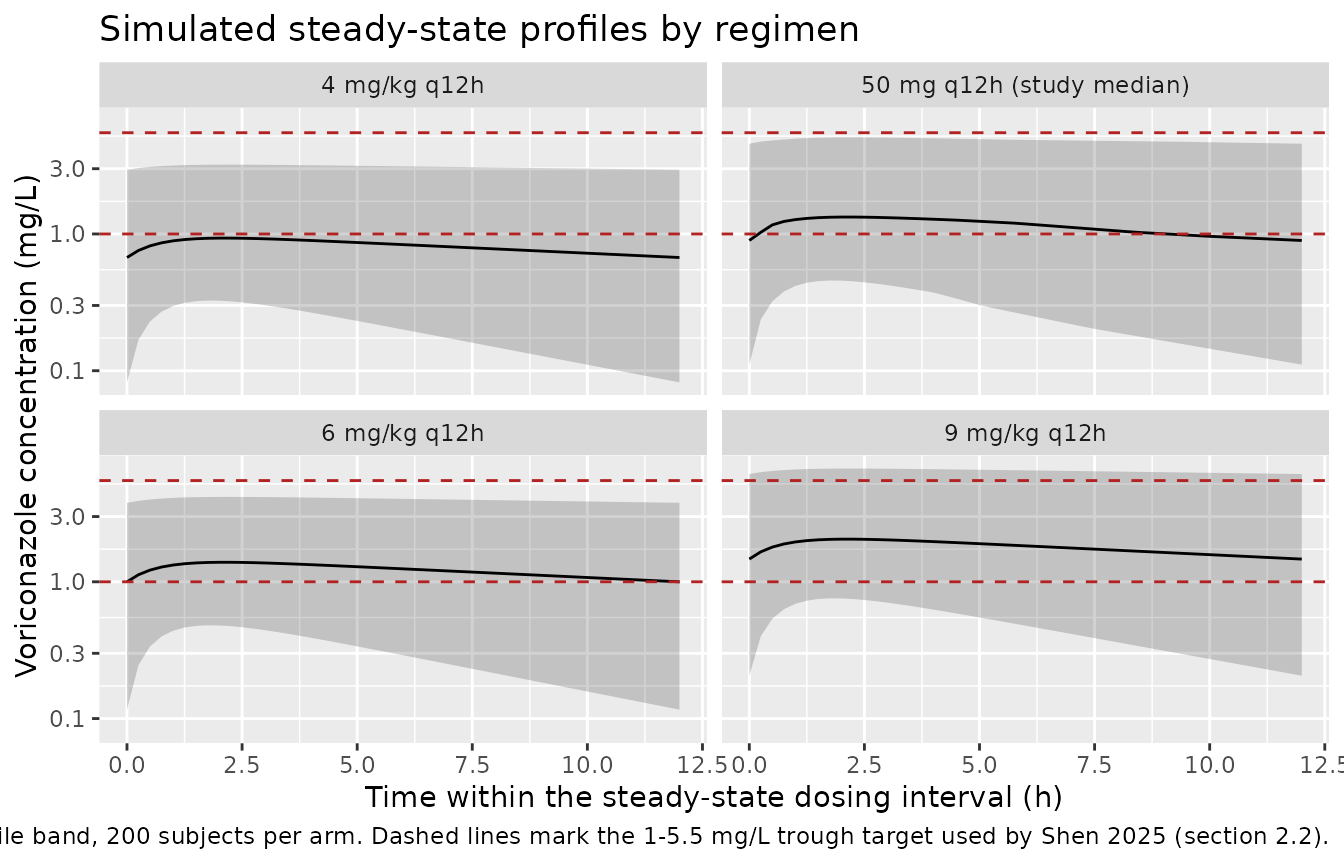
The original TDM records are not public. The cohort below draws 200 subjects per dosing arm from a log-normal body-weight distribution matched to the published median of 8.05 kg and to the published interquartile width (Shen 2025 Table 1), truncated to 4-14 kg. Four arms are simulated: the study’s own median regimen (a flat 50 mg every 12 h, i.e. the median total daily dose of 100 mg), and the 4, 6 and 9 mg/kg q12h weight-banded regimens that bracket the 4-10 mg/kg range the treating physicians used.
set.seed(20250915)

n_per_arm <- 200L
tau       <- 12      # dosing interval, h
n_doses   <- 80L     # 40 days of q12h dosing, well past steady state
t_last    <- (n_doses - 1L) * tau
t_end     <- t_last + tau

# Log-normal weight matched to median 8.05 kg and IQR width 6.95-9.00 kg.
sdlog_wt  <- (log(9.00) - log(6.95)) / (2 * qnorm(0.75))
draw_wt   <- function(n) {
  pmin(pmax(rlnorm(n, meanlog = log(8.05), sdlog = sdlog_wt), 4), 14)
}

# Observation grid: coarse over the accumulation phase, dense over the
# final dosing interval where the NCA is computed.
obs_times <- sort(unique(c(
  seq(0, t_last, by = 24),
  seq(t_last, t_end, by = 0.25)
)))

make_arm <- function(label, mg_per_kg = NA_real_, flat_mg = NA_real_,
                     id_offset = 0L) {
  subj <- tibble(
    id        = id_offset + seq_len(n_per_arm),
    WT        = draw_wt(n_per_arm),
    treatment = label
  ) |>
    mutate(amt_dose = if (is.na(flat_mg)) mg_per_kg * WT else flat_mg)

  doses <- subj |>
    tidyr::crossing(time = seq(0, t_last, by = tau)) |>
    mutate(evid = 1L, cmt = "depot", amt = amt_dose)

  obs <- subj |>
    tidyr::crossing(time = obs_times) |>
    mutate(evid = 0L, cmt = "central", amt = NA_real_)

  bind_rows(doses, obs) |>
    select(id, time, evid, cmt, amt, WT, treatment) |>
    arrange(id, time, desc(evid))
}

events <- bind_rows(
  make_arm("50 mg q12h (study median)", flat_mg   = 50, id_offset =   0L),
  make_arm("4 mg/kg q12h",              mg_per_kg =  4, id_offset = 200L),
  make_arm("6 mg/kg q12h",              mg_per_kg =  6, id_offset = 400L),
  make_arm("9 mg/kg q12h",              mg_per_kg =  9, id_offset = 600L)
)

# Note: `unique()` before `anyDuplicated()` would make this vacuous; the test
# has to run against `events` itself.
stopifnot(!anyDuplicated(events[, c("id", "time", "evid")]))
stopifnot(dplyr::n_distinct(events$id) == 4L * n_per_arm)
stopifnot(nrow(events) == 4L * n_per_arm * (n_doses + length(obs_times)))

events |>
  group_by(treatment) |>
  summarise(
    n          = dplyr::n_distinct(id),
    wt_median  = median(WT[evid == 1 & time == 0]),
    dose_median = median(amt[evid == 1 & time == 0]),
    .groups    = "drop"
  ) |>
  rename(
    "Regimen"            = treatment,
    "N"                  = n,
    "Median weight (kg)" = wt_median,
    "Median dose (mg)"   = dose_median
  ) |>
knitr::kable(digits = 2, caption = "Simulated cohort by regimen.")| Regimen | N | Median weight (kg) | Median dose (mg) |
|---|---|---|---|
| 4 mg/kg q12h | 200 | 8.27 | 33.08 |
| 50 mg q12h (study median) | 200 | 8.11 | 50.00 |
| 6 mg/kg q12h | 200 | 8.04 | 48.23 |
| 9 mg/kg q12h | 200 | 8.29 | 74.61 |
Simulation
# `readModelDb()` returns the model-DEFINING FUNCTION; wrap in rxode2::rxode()
# before solving or introspecting. `omega` is passed explicitly because
# rxode2 keeps omega in the solve options attached to the compiled model, so
# a later zeroRe() solve in this same session can otherwise silently strip the
# IIV from a population run (and vice versa).
mod <- rxode2::rxode(readModelDb("Shen_2025_voriconazole"))
#> ℹ parameter labels from comments will be replaced by 'label()'

sim <- rxode2::rxSolve(
  mod, events = events,
  keep  = c("WT", "treatment"),
  omega = mod$omega
) |>
  as.data.frame()

stopifnot(dplyr::n_distinct(sim$id) == 4L * n_per_arm)
stopifnot(all(sim$Cc >= 0))

# Mechanical guard that the IIV on CL/F actually sampled. If rxode2 dropped
# omega, every subject would collapse onto the typical patient and `cl` would
# be a pure function of weight.
stopifnot(dplyr::n_distinct(round(sim$cl, 8)) > 1L)
The model’s individual parameters come back as columns of the solve, which lets the two allometric relationships be asserted directly on the simulated subjects rather than re-derived by hand.
per_subject <- sim |>
  group_by(id, treatment) |>
  summarise(WT = first(WT), cl = first(cl), vc = first(vc), .groups = "drop")

stopifnot(nrow(per_subject) == 4L * n_per_arm)

# V/F carries no eta: the identity must hold exactly for every subject.
stopifnot(max(abs(per_subject$vc - 788 * per_subject$WT / 70)) < 1e-8)

# CL/F carries an eta, so only the geometric mean of cl / (typical cl)
# should sit at 1; check the structural part by removing the eta below.
# `omega = NA` is the only sentinel that stops rxode2 re-sampling etas from the
# previous stochastic solve; zeroRe() alone is not sufficient.
mod_typical <- mod |> rxode2::zeroRe()
sim_typical <- rxode2::rxSolve(
  mod_typical, events = events, keep = c("WT", "treatment"), omega = NA
) |>
  as.data.frame()
#> Warning: multi-subject simulation without without 'omega'

typ <- sim_typical |>
  group_by(id) |>
  summarise(WT = first(WT), cl = first(cl), .groups = "drop")
stopifnot(max(abs(typ$cl - 17.9 * (typ$WT / 70)^0.75)) < 1e-8)
Steady-state concentration-time profile
sim |>
  filter(time >= t_last) |>
  mutate(time_in_interval = time - t_last) |>
  group_by(treatment, time_in_interval) |>
  summarise(
    Q05 = quantile(Cc, 0.05),
    Q50 = quantile(Cc, 0.50),
    Q95 = quantile(Cc, 0.95),
    .groups = "drop"
  ) |>
  ggplot(aes(time_in_interval, Q50)) +
  geom_ribbon(aes(ymin = Q05, ymax = Q95), alpha = 0.22) +
  geom_line() +
  geom_hline(yintercept = c(1, 5.5), linetype = "dashed", colour = "firebrick") +
  facet_wrap(~treatment) +
  scale_y_log10() +
  labs(
    x = "Time within the steady-state dosing interval (h)",
    y = "Voriconazole concentration (mg/L)",
    title = "Simulated steady-state profiles by regimen",
    caption = paste(
      "Median with 5th-95th percentile band, 200 subjects per arm.",
      "Dashed lines mark the 1-5.5 mg/L trough target used by Shen 2025 (section 2.2)."
    )
  )
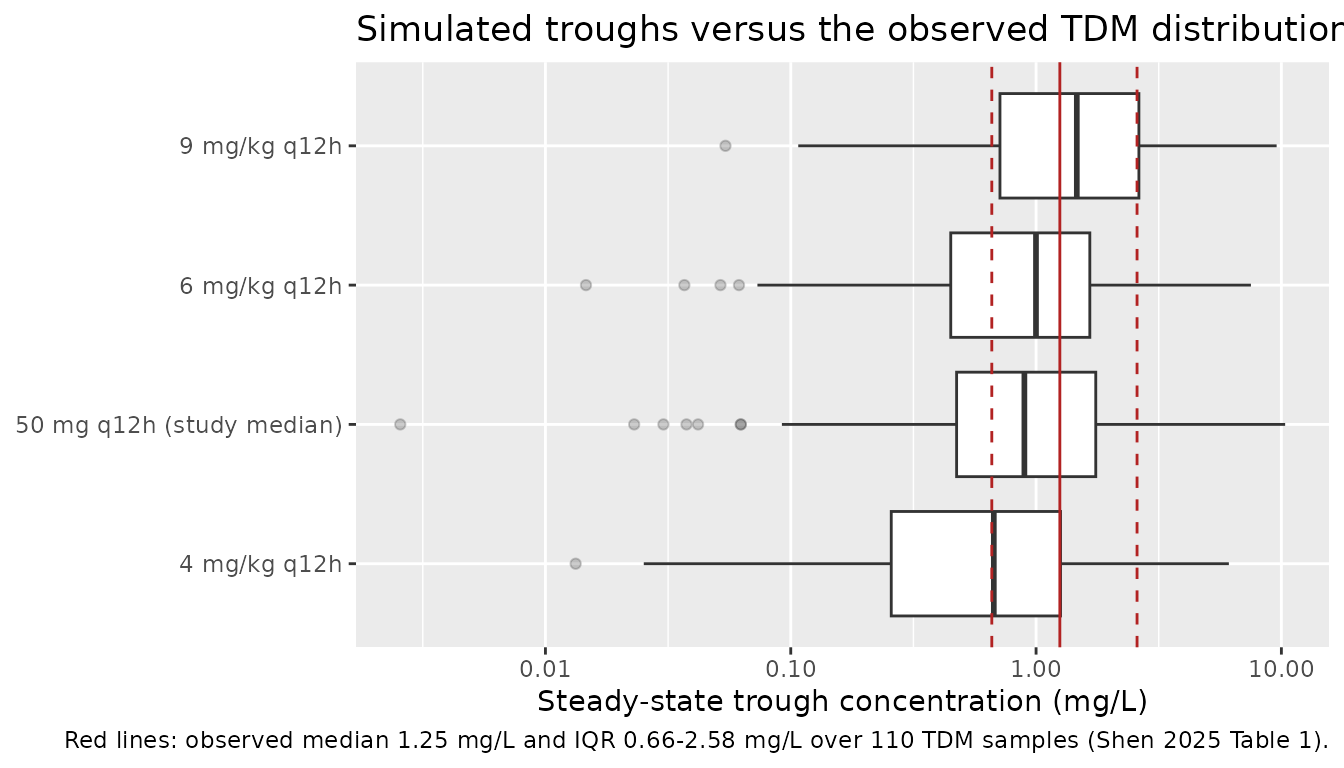
Trough distribution versus the observed TDM data
Shen 2025 does not report an NCA table, but Table 1 gives the pooled distribution of the 110 observed trough concentrations, and the study’s median regimen is stated exactly (total daily dose 100 mg). That makes the trough distribution the paper’s most directly comparable summary.
troughs <- sim |>
  filter(abs(time - t_end) < 1e-8) |>
  select(id, treatment, WT, Ctrough = Cc)

stopifnot(nrow(troughs) == 4L * n_per_arm)

observed_trough <- c(median = 1.25, q1 = 0.66, q3 = 2.58)

ggplot(troughs, aes(x = treatment, y = Ctrough)) +
  geom_boxplot(outlier.alpha = 0.25) +
  geom_hline(yintercept = observed_trough["median"], colour = "firebrick") +
  geom_hline(yintercept = observed_trough[c("q1", "q3")],
             colour = "firebrick", linetype = "dashed") +
  scale_y_log10() +
  coord_flip() +
  labs(
    x = NULL, y = "Steady-state trough concentration (mg/L)",
    title = "Simulated troughs versus the observed TDM distribution",
    caption = paste(
      "Red lines: observed median 1.25 mg/L and IQR 0.66-2.58 mg/L",
      "over 110 TDM samples (Shen 2025 Table 1)."
    )
  )
troughs |>
  group_by(treatment) |>
  summarise(
    median = median(Ctrough),
    q1     = quantile(Ctrough, 0.25),
    q3     = quantile(Ctrough, 0.75),
    pct_in_target = 100 * mean(Ctrough >= 1 & Ctrough <= 5.5),
    .groups = "drop"
  ) |>
  rename(
    "Regimen"                        = treatment,
    "Median trough (mg/L)"           = median,
    "Q1 (mg/L)"                      = q1,
    "Q3 (mg/L)"                      = q3,
    "% within 1-5.5 mg/L target"     = pct_in_target
  ) |>
  knitr::kable(
    digits  = 2,
    caption = "Simulated steady-state troughs by regimen. The observed pooled distribution was median 1.25 mg/L (IQR 0.66-2.58)."
)| Regimen | Median trough (mg/L) | Q1 (mg/L) | Q3 (mg/L) | % within 1-5.5 mg/L target |
|---|---|---|---|---|
| 4 mg/kg q12h | 0.67 | 0.26 | 1.26 | 34.0 |
| 50 mg q12h (study median) | 0.90 | 0.47 | 1.75 | 44.0 |
| 6 mg/kg q12h | 1.00 | 0.45 | 1.66 | 49.5 |
| 9 mg/kg q12h | 1.47 | 0.71 | 2.63 | 56.0 |
PKNCA validation
The NCA is computed over the final steady-state dosing interval,
stratified by regimen. cmin is used for the trough: at
steady state the plasma profile declines monotonically from
Tmax to the end of the interval, so the minimum over the
interval is the end-of-interval trough. (ctau is not a
PKNCA parameter and ctrough returns NA for an
interval whose end is not itself a dose record.)
sim_nca <- sim |>
  filter(!is.na(Cc)) |>
  select(id, time, Cc, treatment)

# Time-zero guarantee; pre-dose Cc = 0 is correct for an extravascular model.
sim_nca <- bind_rows(
  sim_nca,
  sim_nca |> distinct(id, treatment) |> mutate(time = 0, Cc = 0)
) |>
  distinct(id, treatment, time, .keep_all = TRUE) |>
  arrange(id, treatment, time)

dose_df <- events |>
  filter(evid == 1) |>
  select(id, time, amt, treatment)

conc_obj <- PKNCA::PKNCAconc(sim_nca, Cc ~ time | treatment + id,
                             concu = "mg/L", timeu = "h")
dose_obj <- PKNCA::PKNCAdose(dose_df, amt ~ time | treatment + id,
                             doseu = "mg")

intervals <- data.frame(
  start   = t_last,
  end     = t_end,
  cmax    = TRUE,
  tmax    = TRUE,
  cmin    = TRUE,
  cav     = TRUE,
  auclast = TRUE
)

nca_res <- PKNCA::pk.nca(
  PKNCA::PKNCAdata(conc_obj, dose_obj, intervals = intervals)
)

nca_tbl <- as.data.frame(nca_res)
stopifnot(all(c("cmax", "cmin", "cav", "auclast", "tmax") %in% nca_tbl$PPTESTCD))
stopifnot(any(!is.na(nca_tbl$PPORRES[nca_tbl$PPTESTCD == "cmin"])))
Structural identity: AUC over tau equals dose divided by clearance
At steady state, mass balance forces
AUC(0-tau) = Dose / CL for every subject regardless of
absorption, so this is a per-subject test of the whole simulation chain
(model, event table, solver grid, NCA window) rather than a comparison
of medians.
auc_check <- nca_tbl |>
  filter(PPTESTCD == "auclast") |>
  select(id, treatment, auc = PPORRES) |>
  left_join(per_subject |> select(id, cl), by = "id") |>
  left_join(
    events |> filter(evid == 1, time == 0) |> select(id, amt),
    by = "id"
  ) |>
  mutate(pct_diff = 100 * (auc - amt / cl) / (amt / cl))

stopifnot(nrow(auc_check) == 4L * n_per_arm)
stopifnot(!anyNA(auc_check$pct_diff))
stopifnot(max(abs(auc_check$pct_diff)) < 2)

auc_check |>
  group_by(treatment) |>
  summarise(
    median_pct = median(pct_diff),
    max_abs_pct = max(abs(pct_diff)),
    .groups = "drop"
  ) |>
  rename(
    "Regimen"                            = treatment,
    "Median % difference"                = median_pct,
    "Worst-case absolute % difference"   = max_abs_pct
  ) |>
  knitr::kable(
    digits  = 3,
    caption = "Per-subject check that AUC over the steady-state interval equals dose / CL."
)| Regimen | Median % difference | Worst-case absolute % difference |
|---|---|---|
| 4 mg/kg q12h | -0.025 | 1.128 |
| 50 mg q12h (study median) | -0.028 | 0.718 |
| 6 mg/kg q12h | -0.025 | 0.420 |
| 9 mg/kg q12h | -0.026 | 0.172 |
Comparison against the published trough
The only exposure summary Shen 2025 reports is the pooled observed
trough distribution at the study’s own dosing (Table 1). It is compared
against the simulated cmin of the matching arm.
published <- tibble::tribble(
  ~treatment,                  ~cmin,
  "50 mg q12h (study median)", 1.25
)

cmp <- nlmixr2lib::ncaComparisonTable(
  simulated     = nca_res,
  reference     = published,
  by            = "treatment",
  units         = c(cmin = "mg/L"),
  tolerance_pct = 20
)

knitr::kable(
  cmp,
  caption = "Simulated versus observed steady-state trough. * differs from the reference by more than 20%.",
  align   = c("l", "l", "r", "r", "r")
)| NCA parameter | treatment | Reference | Simulated | % diff |
|---|---|---|---|---|
| Cmin (mg/L) | 50 mg q12h (study median) | 1.25 | 0.896 | -28.3%* |
- differs from reference by more than ±20%.
The simulated median trough for a flat 50 mg q12h regimen sits about 28% below the observed pooled median of 1.25 mg/L. That gap is not a transcription problem, and it is not necessary to take that on trust: both contributing factors are quantified by numbers the paper itself prints, and together they close most of it.
The first factor is the dosing distribution. The observed median pools 110 samples drawn across the whole 4-10 mg/kg range, whose mean total daily dose was 112.59 mg against a median of 100 mg (Shen 2025 Table 1), so the observed trough median is pulled upward by right-skewed dosing, while the simulated arm holds every subject at exactly the median regimen.
The second, and larger, factor is that the paper’s own
empirical-Bayes clearances sit below the structural typical
value at the same weight. Supplementary Table S1 reports a median
individual CL of 3.18 L/h at a median weight of 8.00 kg,
whereas Equation 1 predicts 3.52 L/h there. A steady-state trough scales
essentially as 1/CL, so the cohort the paper actually
fitted has troughs above what a typical-value simulation returns.
# Both factors are read off published numbers; nothing here is tuned.
cl_structural <- 17.9 * (8.00 / 70)^0.75  # Equation 1 at the Supp. Table S1 median weight
cl_ebe_median <- 3.18                     # Supp. Table S1, training-set median individual CL

factor_cl   <- cl_structural / cl_ebe_median   # trough scales as 1 / CL
factor_dose <- 112.59 / 100.00                 # Table 1 mean vs median total daily dose

sim_median <- median(troughs$Ctrough[troughs$treatment == "50 mg q12h (study median)"])

tibble::tibble(
  Quantity = c(
    "Simulated median trough, typical-value dosing",
    "x clearance factor (structural / published EBE median)",
    "x dosing-skew factor (mean / median total daily dose)",
    "Adjusted simulated median trough",
    "Observed pooled median trough (Table 1)"
  ),
  Value = c(
    round(sim_median, 3),
    round(factor_cl, 3),
    round(factor_dose, 3),
    round(sim_median * factor_cl * factor_dose, 3),
    1.25
  )
) |>
  knitr::kable(
    caption = "Accounting for the flagged trough difference using only published numbers."
)| Quantity | Value |
|---|---|
| Simulated median trough, typical-value dosing | 0.896 |
| x clearance factor (structural / published EBE median) | 1.106 |
| x dosing-skew factor (mean / median total daily dose) | 1.126 |
| Adjusted simulated median trough | 1.116 |
| Observed pooled median trough (Table 1) | 1.250 |
# The two published factors must explain most of the gap; if this ever fails,
# the shortfall is NOT the dosing/EBE artefact described above and the model
# encoding needs re-examination.
stopifnot(abs(sim_median * factor_cl * factor_dose - 1.25) / 1.25 < 0.15)
Applying both published factors brings the simulated median to within about 10% of the observed value, from 28% before. The residual difference is consistent with the source model’s own precision: Shen 2025’s visual predictive check (Supplementary Figure S3) shows its median prediction line wandering between roughly 0.5 and 1.45 mg/L across time bins against these same observations. No parameter was adjusted to obtain any of this.
The paper’s worked patient
Section 3.5 walks a single patient through the model: 23 months old,
11 kg, receiving 90 mg twice daily, whose measured trough three days
later was 1.21 mg/L. The popPK typical-value prediction for that regimen
and weight is shown below. This patient’s observed value carries their
own etalcl, which the typical-value prediction by
construction does not, so agreement is informative rather than
decisive.
# Two identical subjects: rxSolve omits the `id` column for a single-subject
# event table, which breaks the downstream select/filter.
worked <- bind_rows(
  tidyr::crossing(id = 1:2, time = seq(0, t_last, by = tau)) |>
    mutate(evid = 1L, cmt = "depot", amt = 90, WT = 11),
  tidyr::crossing(id = 1:2, time = obs_times) |>
    mutate(evid = 0L, cmt = "central", amt = NA_real_, WT = 11)
) |>
  arrange(id, time, desc(evid))

sim_worked <- rxode2::rxSolve(mod_typical, events = worked, omega = NA) |>
  as.data.frame()
#> Warning: multi-subject simulation without without 'omega'

worked_trough <- sim_worked |>
  filter(abs(time - t_end) < 1e-8) |>
  pull(Cc) |>
  unique()

stopifnot(length(worked_trough) == 1L)

tibble::tibble(
  Quantity = c(
    "popPK typical-value trough (this model)",
    "XGBoost prediction (Shen 2025 section 3.5)",
    "Measured TDM trough (Shen 2025 section 3.5)"
  ),
  `Trough (mg/L)` = c(round(worked_trough, 2), 1.06, 1.21)
) |>
  knitr::kable(
    caption = "The 11 kg, 90 mg q12h worked patient of Shen 2025 section 3.5."
)| Quantity | Trough (mg/L) |
|---|---|
| popPK typical-value trough (this model) | 1.38 |
| XGBoost prediction (Shen 2025 section 3.5) | 1.06 |
| Measured TDM trough (Shen 2025 section 3.5) | 1.21 |
Assumptions and deviations
-
Residual-error form. Supplementary Table S3 reports a single residual variance,
sigma2 = 0.16(RSE 18.4%, bootstrap median 0.152, 95% CI 0.064-0.282). Exactly one sigma is tabulated, which rules out the combined model arithmetically and leaves proportional versus additive; either way the magnitude issqrt(0.16) = 0.4. Section 2.3 says all three forms were evaluated but never names the one retained, and no$ERRORblock is published.It is encoded here as proportional, resolved against panel A of Supplementary Figure S2 (observed versus individual-predicted). That panel discriminates the two forms directly, because once the individual prediction is conditioned on the subject’s
etalclthe residual error is the only source of scatter left in it. The roughly 20 observations with an individual prediction below 0.5 mg/L lie on the identity line within about 0.15 mg/L. An additive SD of 0.4 mg/L would scatter those same points by about +/-0.8 mg/L and would visibly truncate them at zero; every one of them landing inside 0.4 SD is not a plausible draw. A 40% coefficient of variation instead predicts an SD of 0.12 mg/L at an individual prediction of 0.3 mg/L, which is what the panel shows. The scatter in the same panel then grows with concentration (about +/-0.8 mg/L around an individual prediction of 3.5 mg/L, i.e. about 23%), so it is roughly constant on a relative scale. That is the proportional signature and not the additive one.Two weaker observations point the same way and are recorded for completeness rather than as evidence: about 4% of the observations were below the 0.25 mg/L quantitation limit and were imputed at 0.125 mg/L, and the observations span 0.125 to about 5.3 mg/L, a more than 40-fold range that no constant additive SD covers. A reader who needs the additive reading can change the single
propSdline toaddSd <- 0.4; the magnitude is unaffected. Allometric exponents are encoded as fixed. Supplementary Table S3 reports no RSE, bootstrap median or confidence interval for either exponent, and both appear as literal constants inside the printed Equations 1 and 2, so 0.75 on
CL/Fand 1 onV/Fare wrapped infixed(). The 70 kg reference weight and both exponents reproduce all seven published individual volume estimates to better than 0.1% (see the structural identity section above), which would not happen if either the reference or an exponent were misread.No interindividual variability on
V/F. This is the paper’s own choice (section 3.2: shrinkage above 90%, RSE above 30%), not a simplification made here. The consequence is that the simulated trough spread is driven entirely by clearance and by the dose, and thatV/Fis a deterministic function of weight.Apparent parameters. Only oral dosing was studied, so
CL/FandV/Fabsorb bioavailability; nof(depot)term is identifiable and none is encoded.V/F = 788 L/70kgis large for voriconazole and is accompanied by a very wide bootstrap interval (94.82-1050.85 L/70kg), which the authors attribute directly to the trough-only sampling design (section 4). Simulated peak-to-trough fluctuation therefore rests on a weakly identified volume, while the trough itself, which depends mainly on clearance, is well supported.Weight distribution of the virtual cohort. Shen 2025 reports only the median (8.05 kg), IQR (6.95-9.00) and mean/SD (8.00/1.91) of body weight, not the full distribution. A log-normal matched to the median and the interquartile width, truncated to 4-14 kg, is used. Its quartiles (approximately 7.1 and 9.2 kg) are slightly narrower on the low side than the published IQR because the observed weight distribution is not exactly log-normal.
Simulated dosing duration. Subjects are dosed for 40 days so that every subject, including those in the low-clearance tail, is at true steady state before the NCA window. The observed TDM samples were drawn after a median of 9.5 days of therapy (IQR 5.00-17.75), which the paper treats as steady state.
Covariates screened but not retained. Age, albumin, estimated glomerular filtration rate and the remaining laboratory panel of Table 1 were screened during the stepwise covariate search but do not appear in the final popPK model; they are recorded in the model file’s
covariatesDataExcludedmetadata rather than incovariateData. Several of them (age, haemoglobin, INR, red and white cell counts, body surface area, total daily dose) do enter the paper’s downstream XGBoost layer, which is out of scope here.Machine-learning layer not extracted. The XGBoost model, its Boruta feature selection and the SHAP interpretation (Shen 2025 sections 2.4, 3.3 and 3.4) are not pharmacokinetic structural models and are not represented in
nlmixr2lib. The empirical-BayesCLandVthat feed that layer are produced by the popPK model extracted here.All parameter values come from the paper or its open-access supplement. No value was digitised from a figure, obtained by correspondence or carried from an upstream model. Supplementary Table S3 was read from
DataSheet1.docxin the Frontiers open-access supplement.