Pazopanib PK, liver toxicity and tumor size (Tan 2025)
Source:vignettes/articles/Tan_2025_pazopanib.Rmd
Tan_2025_pazopanib.RmdModel and source
- Citation: Tan Z, Voller S, Yin A, Rieborn A, Gelderblom H, van der Hulle T, Knibbe CAJ, Moes DJAR. Model-Informed Dose Optimization of Pazopanib in Real-World Patients with Cancer. Clin Pharmacokinet. 2025;64(5):715-728. doi:10.1007/s40262-025-01504-5.
- Article: https://doi.org/10.1007/s40262-025-01504-5 (open access)
Tan et al. analysed routine therapeutic-drug-monitoring (TDM) data from adults treated with oral pazopanib at Leiden University Medical Center. They built three linked models, packaged here as four files:
| Model file | Content |
|---|---|
Tan_2025_pazopanib |
One-compartment population PK with a dose-nonlinear relative bioavailability |
Tan_2025_pazopanib_livertox |
Gompertz time-to-first-event model for CTCAE grade >= 2 liver toxicity, with a step increase in hazard while the trough exceeds 34 mg/L |
Tan_2025_pazopanib_tumor_mrcc |
Tumor size (sum of longest diameters, SLD) model for metastatic renal cell carcinoma (mRCC) |
Tan_2025_pazopanib_tumor_sts |
The same tumor size structure fitted separately to soft tissue sarcoma (STS) |
The PK model supplies the daily trough concentration
(CTROUGH) that drives the liver-toxicity hazard. The tumor
models have no exposure dependence: the authors tested trough, Cmax and
dose on the decay rate and kept none of them.
Population
132 unique patients (93 mRCC, 39 STS) were treated between 2014 and 2023. Patients who interrupted pazopanib for more than 6 months were entered twice, which gives 135 “individuals” (96 mRCC, 39 STS; Table 1). Median age was 67 years (range 21-89), median weight 79 kg (45-130), and 50 of 135 were female. The median starting dose was 800 mg once daily (range 200-800) and the median dose during treatment 600 mg (200-1000), taken fasted. Race was not reported.
- PK: 460 plasma concentrations (326 troughs, sampled 20-28 h after the dose), median 3 per patient.
- Liver toxicity: 27 of 135 patients (20%) had a grade >= 2 ALT, AST or alkaline phosphatase elevation within 1 year.
- Tumor size: 111 patients had a baseline SLD and at least one on-treatment CT scan (403 SLD records: 322 mRCC, 81 STS). Median baseline SLD was 79 mm in mRCC and 88 mm in STS.
The same information is available programmatically via
readModelDb("Tan_2025_pazopanib")()$population (and the
three companion files).
Source trace
Every ini() value carries an in-file comment pointing to
its source. The supplement prints all four NONMEM control streams, which
confirm the structures and the final values.
| Model / parameter | Value | Source location |
|---|---|---|
| PK: one compartment, first-order absorption, linear elimination | n/a | Results ‘POPPK Model’; supplement PK control stream (ADVAN2 TRANS2) |
lka |
log(0.976) 1/h, fixed | Table 2 ‘Ka’ 0.976 FIX (from Ozbey 2021) |
lcl |
log(0.497) L/h | Table 2 ‘CL/F’ |
lvc |
log(46.1) L | Table 2 ‘V/F’ |
lfdepot |
log(1), fixed | Table 2 ‘TVF1’ 1 FIX |
e_dose_fdepot |
0.42 | Table 2 ‘EXP’ |
f(depot) = exp(lfdepot + etalfdepot) * (200 / DOSE)^e_dose_fdepot |
n/a | Table 2 equation row; control stream
F1 = THETA(6)*EXP(ETA(2))*FCOV
|
etalvc |
0.765^2 | Table 2 ‘IIV_V/F’ 76.5% (control stream $OMEGA
0.58) |
etalfdepot |
0.342^2 | Table 2 ‘IIV_F1’ 34.2% (control stream $OMEGA
0.12) |
propSd, addSd
|
0.24, 4.71 mg/L | Table 2 residual-error rows; control stream
W = SQRT(THETA(4)**2*IPRED**2 + THETA(5)**2)
|
Toxicity: Gompertz hazard
lam * RF * exp(shape * t)
|
n/a | Methods Eqs. 2-3, 6; supplement TTE control stream
$DES
|
llam_haz |
log(0.0021) 1/day | Table 3 ‘Lamda’ |
shape_haz |
-0.012 1/day | Table 3 ‘SHAPE’ |
e_ctrough_haz |
1.21 | Table 3 ‘Cmin,ss coefficient’ (exp(1.21) = 3.35) |
ctrough_cut |
34 mg/L, fixed | Table 3 footnote; control stream IF(trough.GT.34);
Supplementary Table S1 |
Tumor:
dSLD/dt = p * SLD - kkill * exp(-res * t) * SLD
|
n/a | Fig. 2, Eqs. 7-8; supplement tumor control streams
$DES
|
tumor_size(0) = TUM_SLD |
n/a | Methods; control stream A_0(3) = BASE
|
kkill = 0 in the resistant class |
n/a | Fig. 2 legend; control stream
IF(MIXNUM.EQ.2) KD = THETA(2) (0 FIX) |
mRCC lp, lkkill, lres
|
log(0.0005), log(0.004), log(0.008) 1/day | Table 4 mRCC column |
mRCC etalp, etalkkill
|
1.30^2, 0.54^2 | Table 4 ‘IIV_KG’ 130%, ‘IIV_KD’ 54% (control stream
$OMEGA 1.69, 0.29) |
mRCC propSd, addSd
|
0.138, 1.24 mm | Table 4 residual-error rows |
| mRCC resistant fraction | 0.27 | Table 4 ‘Subpopulation of primary resistance’; control stream
P(1) = THETA(7) = 0.73 |
STS lp, lkkill, lres
|
log(0.0086), log(0.008), log(0.0003) 1/day | Table 4 STS column |
STS etalkkill
|
0.017 | Table 4 ‘IIV_KD’ 13%; control stream $OMEGA 0.017 (IIV
on KG 0 FIX) |
STS propSd, addSd
|
0.166, 8.1 mm | Table 4 residual-error rows |
| STS resistant fraction | 0.134 | Table 4; control stream P(1) = 0.866 |
Pharmacokinetics
Virtual cohort and simulation
Figure 4a of the paper compares three fixed starting regimens: 400, 600 and 800 mg once daily. The cohort below has 200 subjects per regimen, dosed for a full year so the same simulation also supplies the daily troughs for the liver-toxicity model. Concentrations are sampled just before each dose (the daily trough) and hourly over days 29-30 for the steady-state profile.
n_per_arm <- 200L
doses <- c(400, 600, 800)
n_days <- 365L

make_pk_arm <- function(dose, id_offset) {
  ids <- id_offset + seq_len(n_per_arm)
  dose_rows <- data.frame(
    id = ids, time = 0, amt = dose, evid = 1L, cmt = "depot",
    ii = 24, addl = n_days - 1L
  )
  obs_times <- sort(unique(c(
    24 * seq_len(n_days) - 0.01, # daily troughs, just before the next dose
    seq(696, 720, by = 1) # day 29-30 steady-state profile
  )))
  obs_rows <- expand.grid(id = ids, time = obs_times) |>
    mutate(amt = 0, evid = 0L, cmt = "central", ii = 0, addl = 0L)
  bind_rows(dose_rows, obs_rows) |>
    mutate(DOSE = dose, arm = paste(dose, "mg QD")) |>
    arrange(id, time, desc(evid))
}

pk_events <- bind_rows(
  make_pk_arm(400, 0L),
  make_pk_arm(600, n_per_arm),
  make_pk_arm(800, 2L * n_per_arm)
)
stopifnot(!anyDuplicated(unique(pk_events[, c("id", "time", "evid")])))
mod_pk <- readModelDb("Tan_2025_pazopanib")
rxode2::rxSetSeed(20250425)
pk_sim <- rxode2::rxSolve(mod_pk, events = pk_events, keep = "arm") |>
  as.data.frame()
#> ℹ parameter labels from comments will be replaced by 'label()'
Steady-state profiles (Figure 4a)
pk_ss <- pk_sim |>
  filter(time >= 600, time <= 720) |>
  group_by(arm, time) |>
  summarise(
    med = median(Cc), lo = quantile(Cc, 0.05), hi = quantile(Cc, 0.95),
    .groups = "drop"
  )
ggplot(pk_ss, aes(time / 24, med)) +
  geom_ribbon(aes(ymin = lo, ymax = hi), alpha = 0.3) +
  geom_line() +
  geom_hline(yintercept = 20.5, linetype = "dashed", colour = "blue") +
  geom_hline(yintercept = 34, linetype = "dashed", colour = "red") +
  facet_wrap(~arm, ncol = 1) +
  labs(
    x = "Time (day)", y = "Pazopanib concentration (mg/L)",
    caption = "Replicates Figure 4a of Tan 2025: median and 90% prediction interval."
  )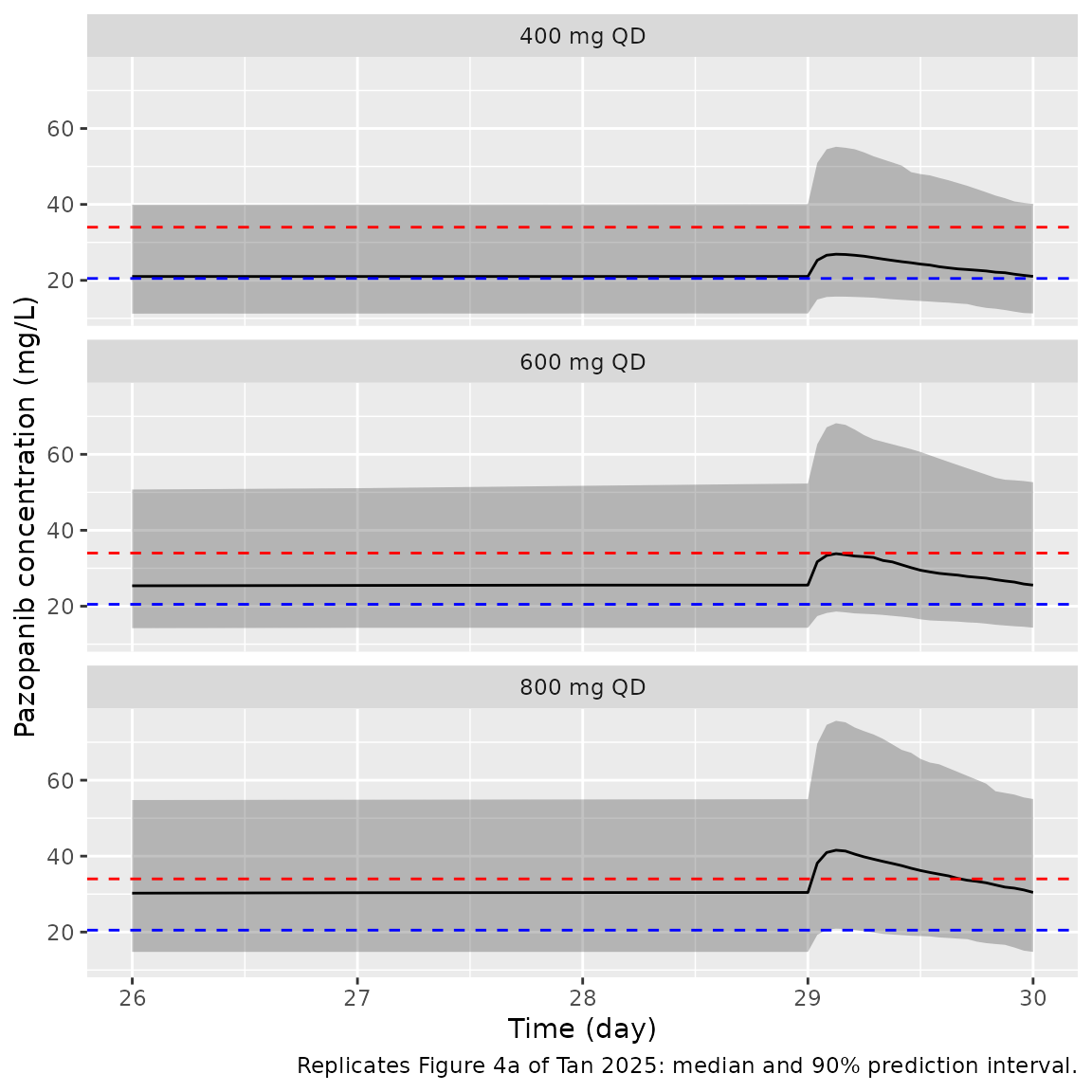
The paper states that the 600 mg regimen keeps the steady-state trough at or above the 20.5 mg/L efficacy threshold in 76% of simulated individuals.
trough_ss <- pk_sim |>
  filter(abs(time - (30 * 24 - 0.01)) < 1e-6) |>
  group_by(arm) |>
  summarise(
    `Median trough (mg/L)` = signif(median(Cc), 3),
    `Trough >= 20.5 mg/L (%)` = round(100 * mean(Cc >= 20.5)),
    `Trough > 34 mg/L (%)` = round(100 * mean(Cc > 34)),
    .groups = "drop"
  ) |>
  rename(Regimen = arm)
knitr::kable(trough_ss, caption = "Simulated day-30 trough by regimen.")| Regimen | Median trough (mg/L) | Trough >= 20.5 mg/L (%) | Trough > 34 mg/L (%) |
|---|---|---|---|
| 400 mg QD | 21.0 | 52 | 14 |
| 600 mg QD | 25.6 | 72 | 24 |
| 800 mg QD | 30.5 | 86 | 36 |
pct_600 <- trough_ss$`Trough >= 20.5 mg/L (%)`[trough_ss$Regimen == "600 mg QD"]
# A cohort-level proportion of 200 subjects (binomial SE about 3 points); the
# bounds catch a wrong F1 exponent or CL, which move it by tens of points.
stopifnot(pct_600 > 60, pct_600 < 95)
The simulated proportion at 600 mg (72%) is close to the 76% the
paper reports. The simulated median troughs are about 21, 26 and 31 mg/L
for 400, 600 and 800 mg. Read from Figure 4a, the published medians are
about 21, 28 and 30 mg/L, with the 600 and 800 mg curves nearly
overlapping. Because bioavailability falls with dose as
(200 / DOSE)^0.42, doubling the dose from 400 to 800 mg
raises exposure by only about 50%.
PKNCA validation
The paper reports no NCA, so the check is against the closed form. At
steady state the AUC over one dosing interval is
F * Dose / (CL/F), with F = (200 / Dose)^0.42.
The typical-value simulation (random effects zeroed) must reproduce
it.
pk_typ_events <- bind_rows(lapply(seq_along(doses), function(i) {
  make_pk_arm(doses[i], (i - 1L) * n_per_arm) |> filter(id == min(id))
}))
pk_typ <- rxode2::rxSolve(rxode2::zeroRe(mod_pk), events = pk_typ_events, keep = "arm") |>
  as.data.frame()
#> ℹ parameter labels from comments will be replaced by 'label()'
#> ℹ omega/sigma items treated as zero: 'etalvc', 'etalfdepot'
#> Warning: multi-subject simulation without without 'omega'

conc_df <- pk_typ |>
  filter(time >= 696, time <= 720, !is.na(Cc)) |>
  mutate(treatment = arm) |>
  select(id, time, Cc, treatment)
# The interval dose is the one given at 696 h (start of day 30).
dose_df <- pk_typ_events |>
  filter(evid == 1) |>
  transmute(id, time = 696, amt, treatment = arm)

conc_obj <- PKNCA::PKNCAconc(conc_df, Cc ~ time | treatment + id)
dose_obj <- PKNCA::PKNCAdose(dose_df, amt ~ time | treatment + id)
intervals <- data.frame(start = 696, end = 720, auclast = TRUE, cmax = TRUE, cmin = TRUE, tmax = TRUE)
nca_res <- PKNCA::pk.nca(PKNCA::PKNCAdata(conc_obj, dose_obj, intervals = intervals))

nca_tab <- as.data.frame(nca_res$result) |>
  select(treatment, PPTESTCD, PPORRES) |>
  pivot_wider(names_from = PPTESTCD, values_from = PPORRES) |>
  mutate(
    dose = as.numeric(sub(" mg QD", "", treatment)),
    auc_closed = (200 / dose)^0.42 * dose / 0.497,
    pct_diff = 100 * (auclast / auc_closed - 1)
  )
nca_tab |>
  transmute(
    Regimen = treatment,
    "Cmax (mg/L)" = signif(cmax, 3),
    "Tmax (h)" = signif(tmax, 3),
    "Cmin (mg/L)" = signif(cmin, 3),
    "AUCtau PKNCA (mg*h/L)" = signif(auclast, 4),
    "AUCtau closed form (mg*h/L)" = signif(auc_closed, 4),
    "Difference (%)" = round(pct_diff, 2)
  ) |>
knitr::kable(caption = "Typical-value steady-state NCA (day 29-30) versus the closed form.")| Regimen | Cmax (mg/L) | Tmax (h) | Cmin (mg/L) | AUCtau PKNCA (mg*h/L) | AUCtau closed form (mg*h/L) | Difference (%) |
|---|---|---|---|---|---|---|
| 400 mg QD | 27.5 | 3 | 22.2 | 600.8 | 601.5 | -0.13 |
| 600 mg QD | 34.8 | 3 | 28.1 | 760.0 | 761.0 | -0.13 |
| 800 mg QD | 41.1 | 3 | 33.2 | 898.1 | 899.2 | -0.13 |
Liver toxicity
Closed-form check
With a constant trough the Gompertz cumulative hazard has a closed
form, H(t) = lambda * RF / shape * (exp(shape * t) - 1),
with RF = exp(1.21) above 34 mg/L and 1 otherwise. The
model must reproduce it exactly.
mod_tox <- readModelDb("Tan_2025_pazopanib_livertox")
tox_check_events <- expand.grid(id = 1:2, time = seq(0, 365, by = 5)) |>
  mutate(evid = 0L, CTROUGH = ifelse(id == 1, 25, 40)) |>
  arrange(id, time)
tox_check <- rxode2::rxSolve(mod_tox, events = tox_check_events, keep = "CTROUGH") |>
  as.data.frame() |>
  mutate(
    rf = ifelse(CTROUGH > 34, exp(1.21), 1),
    sur_closed = exp(-0.0021 * rf / -0.012 * (exp(-0.012 * time) - 1))
  )
#> Warning: multi-subject simulation without without 'omega'
stopifnot(max(abs(tox_check$sur - tox_check$sur_closed)) < 1e-5)
tox_check |>
  filter(time == 365) |>
  transmute(
    "Constant trough (mg/L)" = CTROUGH,
    "Toxicity-free survival at 365 days" = signif(sur, 3),
    "Closed form" = signif(sur_closed, 3)
  ) |>
knitr::kable()| Constant trough (mg/L) | Toxicity-free survival at 365 days | Closed form |
|---|---|---|
| 25 | 0.841 | 0.841 |
| 40 | 0.560 | 0.560 |
The two constant-trough curves are the typical-value counterparts of the survival VPC in Figure 1. Below the cutoff the model gives 84% toxicity-free survival at one year, which matches the observed Kaplan-Meier curve in Figure 1a (about 84%). Above the cutoff it gives 56%, inside the wide prediction interval of Figure 1b, where the observed curve ends near 42% after a small number of patients.
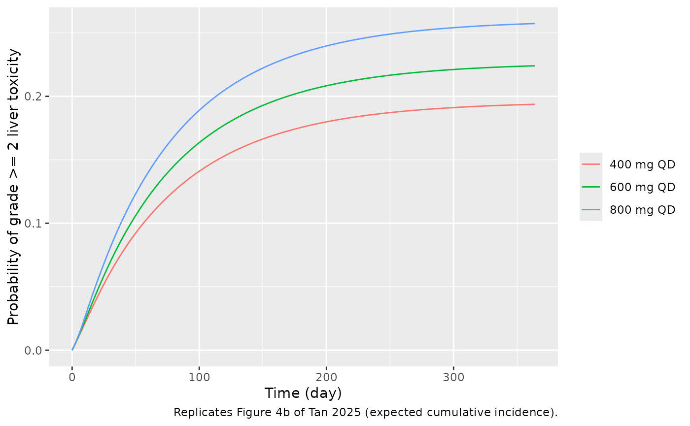
Toxicity probability by starting dose (Figure 4b)
Each simulated subject’s daily trough from the PK simulation above is
passed to the toxicity model as the time-varying CTROUGH
column. The trough recorded on day d is the concentration
just before the dose that starts day d + 1.
tox_events <- pk_sim |>
  filter(abs(time - (24 * round(time / 24) - 0.01)) < 1e-6) |>
  transmute(id, arm, time = round(time / 24) - 1, CTROUGH = Cc, evid = 0L) |>
  filter(time >= 0, time <= 365) |>
  arrange(id, time)
tox_sim <- rxode2::rxSolve(mod_tox, events = tox_events, keep = "arm") |>
  as.data.frame()
#> Warning: multi-subject simulation without without 'omega'

tox_curve <- tox_sim |>
  group_by(arm, time) |>
  summarise(prob_tox = 1 - mean(sur), .groups = "drop")

ggplot(tox_curve, aes(time, prob_tox, colour = arm)) +
  geom_line() +
  labs(
    x = "Time (day)", y = "Probability of grade >= 2 liver toxicity", colour = NULL,
    caption = "Replicates Figure 4b of Tan 2025 (expected cumulative incidence)."
  )
tox_365 <- tox_curve |>
  filter(time == max(time)) |>
  mutate(published = c(0.21, 0.16, 0.37)[match(arm, paste(doses, "mg QD"))])
tox_365 |>
  transmute(
    Regimen = arm,
    "Simulated probability at 1 year" = round(prob_tox, 3),
    "Figure 4b (read from plot)" = published
  ) |>
knitr::kable()| Regimen | Simulated probability at 1 year | Figure 4b (read from plot) |
|---|---|---|
| 400 mg QD | 0.194 | 0.21 |
| 600 mg QD | 0.224 | 0.16 |
| 800 mg QD | 0.257 | 0.37 |
p_tox <- setNames(tox_365$prob_tox, tox_365$arm)
# Expected (not event-sampled) incidence over 200 subjects: monotone in dose
# and bounded by the two constant-trough closed forms (0.16 and 0.44).
stopifnot(
  p_tox[["800 mg QD"]] > p_tox[["600 mg QD"]],
  p_tox[["600 mg QD"]] > p_tox[["400 mg QD"]],
  all(p_tox > 0.15), all(p_tox < 0.45)
)
The simulated one-year risks at 400 and 600 mg are close to the
published values (within about 0.07), but the 800 mg risk is lower than
the published 0.37, and the published order of 400 mg (0.21) above 600
mg (0.16) is not reproduced. The packaged model cannot reach 0.37 at 800
mg with these troughs. Even a subject whose trough stays above 34 mg/L
for the whole year has a one-year risk of only 0.44 (the closed-form
check above), so 0.37 would need roughly three quarters of the cohort
above the cutoff. The paper’s own Figure 4a puts the 800 mg median
trough near 30 mg/L, which means fewer than half of the subjects are
above 34 mg/L. Passing the troughs with their PK residual error (the
sim column) as CTROUGH raises the 800 mg risk
by only about 0.01. The model hazard rises with the trough and the
trough rises with the dose, so the published 400 / 600 mg inversion
points to Monte Carlo noise in the paper’s event-sampled curves. The
parameters were not adjusted to close these gaps.
Tumor size
Closed-form check
The tumor ODE is linear in SLD, so for fixed parameters
log(SLD(t) / SLD(0)) = p * t - kkill / res * (1 - exp(-res * t)),
with kkill = 0 in the primary-resistant class. The relative
change does not depend on the baseline SLD.
mod_mrcc <- readModelDb("Tan_2025_pazopanib_tumor_mrcc")
mod_sts <- readModelDb("Tan_2025_pazopanib_tumor_sts")
tumor_check_events <- expand.grid(id = 1:2, time = seq(0, 360, by = 30)) |>
  mutate(evid = 0L, cmt = "tumor_size", TUM_SLD = 80, MIX_PRIM_RESIST = id - 1L) |>
  arrange(id, time)
closed_pct <- function(time, p, kkill, res, resist) {
  100 * (exp(p * time - (1 - resist) * kkill / res * (1 - exp(-res * time))) - 1)
}
tumor_check <- bind_rows(
  rxode2::rxSolve(rxode2::zeroRe(mod_mrcc), events = tumor_check_events, keep = "MIX_PRIM_RESIST") |>
    as.data.frame() |>
    mutate(tumor = "mRCC", closed = closed_pct(time, 0.0005, 0.004, 0.008, MIX_PRIM_RESIST)),
  rxode2::rxSolve(rxode2::zeroRe(mod_sts), events = tumor_check_events, keep = "MIX_PRIM_RESIST") |>
    as.data.frame() |>
    mutate(tumor = "STS", closed = closed_pct(time, 0.0086, 0.008, 0.0003, MIX_PRIM_RESIST))
) |>
  mutate(pct = 100 * (tumor_size / 80 - 1))
#> ℹ parameter labels from comments will be replaced by 'label()'
#> ℹ omega/sigma items treated as zero: 'etalp', 'etalkkill'
#> Warning: multi-subject simulation without without 'omega'
#> ℹ parameter labels from comments will be replaced by 'label()'
#> ℹ omega/sigma items treated as zero: 'etalkkill'
#> Warning: multi-subject simulation without without 'omega'
stopifnot(max(abs(tumor_check$pct - tumor_check$closed)) < 0.01)
tumor_check |>
  filter(time == 360) |>
  transmute(
    Tumor = tumor,
    Class = ifelse(MIX_PRIM_RESIST == 1, "primary resistant", "primary sensitive"),
    "SLD change at day 360 (%)" = round(pct, 1)
  ) |>
knitr::kable()| Tumor | Class | SLD change at day 360 (%) |
|---|---|---|
| mRCC | primary sensitive | -25.3 |
| mRCC | primary resistant | 19.7 |
| STS | primary sensitive | 44.2 |
| STS | primary resistant | 2110.9 |
Population tumor size over time (Figure 4c)
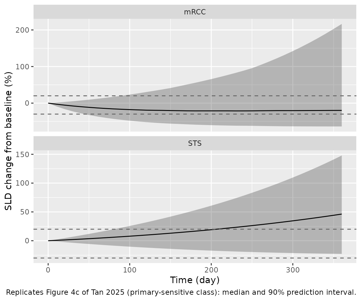
Figure 4c shows the median and 90% prediction interval of the SLD change from baseline. Its curves match the primary-sensitive class rather than the full mixture:
- The mRCC median ends near -22% and the band tops out near 0%.
- The STS median ends between +30% and +60% (one curve per dose, which differ only by Monte Carlo noise) and the band reaches about +165%.
A primary-resistant STS subject grows more than 20-fold in a year (the closed-form table above). With 13.4% of the cohort in that class, the 95th percentile of a full-mixture simulation would lie far above +165%. The cohort below therefore simulates 200 sensitive subjects per tumor type with full inter-individual variability for the comparison, and a second cohort with the class drawn from a Bernoulli distribution with the Table 4 probability (0.27 mRCC, 0.134 STS) shows the full mixture. Baseline SLD is drawn log-normally around the Table 1 medians. It does not affect the percentage change, but it makes the absolute SLD realistic.
set.seed(20250425)
make_tumor_cohort <- function(p_resist, sld_median) {
  subj <- data.frame(
    id = seq_len(n_per_arm),
    MIX_PRIM_RESIST = rbinom(n_per_arm, 1, p_resist),
    TUM_SLD = sld_median * exp(rnorm(n_per_arm, 0, 0.6))
  )
  expand.grid(id = subj$id, time = seq(0, 360, by = 10)) |>
    left_join(subj, by = "id") |>
    mutate(evid = 0L, cmt = "tumor_size") |>
    arrange(id, time)
}
sim_tumor <- function(mod, events, tumor, population) {
  rxode2::rxSolve(mod, events = events, keep = "TUM_SLD") |>
    as.data.frame() |>
    mutate(tumor = tumor, population = population)
}
rxode2::rxSetSeed(20250425)
tumor_sim <- bind_rows(
  sim_tumor(mod_mrcc, make_tumor_cohort(0, 79), "mRCC", "Primary sensitive"),
  sim_tumor(mod_sts, make_tumor_cohort(0, 88), "STS", "Primary sensitive"),
  sim_tumor(mod_mrcc, make_tumor_cohort(0.27, 79), "mRCC", "Full mixture"),
  sim_tumor(mod_sts, make_tumor_cohort(0.134, 88), "STS", "Full mixture")
) |>
  mutate(pct = 100 * (tumor_size / TUM_SLD - 1))
#> ℹ parameter labels from comments will be replaced by 'label()'
#> ℹ parameter labels from comments will be replaced by 'label()'

tumor_summ <- tumor_sim |>
  group_by(population, tumor, time) |>
  summarise(
    med = median(pct), lo = quantile(pct, 0.05), hi = quantile(pct, 0.95),
    .groups = "drop"
  )
ggplot(
  tumor_summ |> filter(population == "Primary sensitive"),
  aes(time, med)
) +
  geom_ribbon(aes(ymin = lo, ymax = hi), alpha = 0.3) +
  geom_line() +
  geom_hline(yintercept = c(-30, 20), linetype = "dashed", colour = "grey40") +
  facet_wrap(~tumor, ncol = 1, scales = "free_y") +
  labs(
    x = "Time (day)", y = "SLD change from baseline (%)",
    caption = paste(
      "Replicates Figure 4c of Tan 2025 (primary-sensitive class):",
      "median and 90% prediction interval."
    )
  )
tab_360 <- tumor_summ |>
  filter(time == 360) |>
  arrange(tumor, desc(population))
tab_360 |>
  transmute(
    Tumor = tumor,
    Population = population,
    "Median (%)" = round(med),
    "5th percentile (%)" = round(lo),
    "95th percentile (%)" = round(hi)
  ) |>
  knitr::kable(caption = paste(
    "SLD change from baseline at day 360. Figure 4c shows a median near -22%",
    "(band about -35% to 0%) for mRCC and +30% to +60% (band about -35% to",
    "+165%) for STS."
))| Tumor | Population | Median (%) | 5th percentile (%) | 95th percentile (%) |
|---|---|---|---|---|
| STS | Primary sensitive | 46 | -23 | 148 |
| STS | Full mixture | 46 | -19 | 2111 |
| mRCC | Primary sensitive | -20 | -64 | 216 |
| mRCC | Full mixture | -10 | -57 | 168 |
med_sens <- tab_360 |> filter(population == "Primary sensitive")
med_mrcc <- med_sens$med[med_sens$tumor == "mRCC"]
med_sts <- med_sens$med[med_sens$tumor == "STS"]
# Medians of 200 subjects; the bounds bracket the Figure 4c medians and still
# separate shrinkage (mRCC) from growth (STS), which a swapped or
# mis-transcribed rate would reverse.
stopifnot(med_mrcc < -10, med_mrcc > -40, med_sts > 20, med_sts < 80)
The sensitive-class medians reproduce Figure 4c. In mRCC the median
tumor shrinks and then levels off, because the drug-induced decay wanes
with an acquired-resistance half-life of about 87 days
(log(2) / 0.008). In STS the growth rate is already higher
than the decay rate at the start, so the median tumor grows throughout
the year. The simulated mRCC 90% band is much wider than the published
one, mainly from the 130% CV on the growth rate KG. The published band
is narrower than that IIV implies, so the paper’s simulation may not
have sampled every random effect; the paper does not say. Including the
primary-resistant class moves the mRCC median towards no change, and
stretches the STS upper tail to the resistant class’s twenty-fold
growth. The authors simulated all three starting doses with the same
tumor model, because the model has no exposure dependence.
Assumptions and deviations
-
IIV variances. Tables 2 and 4 report
inter-individual variability as
CV% = sqrt(omega). The control-stream$OMEGAvalues confirm this: 0.58 gives 76.2% against the printed 76.5%, and 1.69 gives 130%. The variances in the model files are the squared table values (for STSIIV_KD, the control-stream value 0.017). -
No IIV on CL/F. The Results text says IIV on CL/F,
V/F and F1 were estimated, but Table 2 and the control stream contain
IIV only on V/F and F1 (
CL = THETA(1)). The model follows the table and the control stream. -
Table 2 units. Table 2 labels
Kain “h”; the unit is 1/h (Ozbey 2021 reports 0.976 1/h). -
Toxicity model has no residual error. The TTE model
was fitted by likelihood with no random effects
(
$OMEGA 0 FIXon lambda). TheaddSd_surplaceholder is fixed to 0.001 so the model compiles; it is not from the paper. -
Cutoff direction. The Results text says “>= 34
mg/L” in one place and the abstract and control stream say “> 34”.
The model uses the control stream (
trough.GT.34). - Trough input. The paper derived the daily trough from each patient’s empirical-Bayes PK parameters and real dosing history. Here it comes from simulated PK subjects on fixed regimens without TDM dose adjustment.
-
Mixture class as a covariate. The NONMEM
$MIXTUREclass is supplied as the binary columnMIX_PRIM_RESIST. Its population probability (0.27 mRCC, 0.134 STS) is documented incovariateDatarather than carried as anini()parameter, and must be drawn per subject for population simulation. - Tumor-model populations. The paper does not split the 111 tumor-size patients by tumor type, so the demographic fields of the two tumor files describe the whole mRCC and STS PK cohorts. Table 1 lists 69 male / 30 female in the mRCC column, which sums to 99 rather than 96; the female share is computed from those printed counts.
- Figure readings. The Figure 4 comparison values were read from the plot by eye; they are approximate.
- Figure 4c population. The paper does not say which subpopulation Figure 4c shows. The published medians and bands match the primary-sensitive class (see the tumor section), so that class is the comparison here.