Liposomal amphotericin B (Stott 2022)

Model and source

ui <- rxode2::rxode(readModelDb("Stott_2022_amphotericinB_liposomal"))
#> ℹ parameter labels from comments will be replaced by 'label()'

• Citation: Stott KE, Moyo M, Ahmadu A, Kajanga C, Gondwe E, Chimang’anga W, Chasweka M, Leeme TB, Molefi M, Chofle A, Bidwell G, Changalucha J, Unsworth J, Jimenez-Valverde A, Lawrence DS, Mwandumba HC, Lalloo DG, Harrison TS, Jarvis JN, Hope W, Martson AG. Population pharmacokinetics of liposomal amphotericin B in adults with HIV-associated cryptococcal meningoencephalitis. J Antimicrob Chemother. 2023;78(1):276-283. doi:10.1093/jac/dkac389
• Description: Two-compartment IV-infusion population PK model for liposomal amphotericin B (AmBisome) in adults with HIV-associated cryptococcal meningoencephalitis given high-dose, short-course regimens (AMBITION-cm Phase II and III), with no covariates; disposition is written with explicit k12 / k21 micro-constants and no q / vp pair, so solve it with rxSolve(useLinCmt = FALSE) or the peripheral compartment is silently discarded (Stott 2022)
• Article: https://doi.org/10.1093/jac/dkac389

Stott 2022 pooled the pharmacokinetic substudies of the Phase II and Phase III AMBITION-cm trials of high-dose, short-course liposomal amphotericin B (AmBisome) for HIV-associated cryptococcal meningoencephalitis and fitted the data with the nonparametric adaptive grid (NPAG) algorithm of Pmetrics 1.9.7. A two-compartment model with a zero-order infusion into the central compartment and first-order elimination was retained: a third compartment and Michaelis-Menten elimination did not improve the fit. No covariate was retained. The same paper also reports an exposure-toxicity logistic regression and a meta-analysis of clinical outcomes after AmBisome monotherapy; neither is encodable from the printed values (see Assumptions and deviations).

Solve this model with useLinCmt = FALSE. Its model() block exposes the micro-constants k12 and k21 (the paper’s KCP and KPC) rather than a q / vp pair, so a linCmt() conversion has no well-formed two-compartment macro-parameterisation to build.

Population

The model was fitted to 87 adults with HIV-associated cryptococcal meningoencephalitis: 56 from all four arms of the Phase II trial (Princess Marina Hospital, Gaborone, Botswana and Bugando Medical Centre and Sekou Toure Hospital, Mwanza, Tanzania; January 2015 to August 2016) and 31 from the single-dose intervention arm of the Phase III trial (Queen Elizabeth Central Hospital, Blantyre, Malawi; November 2018 to October 2019). Table 1 gives 55 men and 32 women, a median age of 37 years (IQR 32-43), a median weight of 52.0 kg (IQR 46.5-58.7), a median serum creatinine of 64.0 umol/L (IQR 58.0-87.2) and a median CD4+ count of 30 cells/mm^3 (IQR 12-60).

AmBisome was infused over 2 h after pre-hydration. The Phase II arms were 3 mg/kg/day for 14 days; 10 mg/kg on day 1 only; 10 mg/kg on day 1 plus 5 mg/kg on day 3; and 10 mg/kg on day 1 plus 5 mg/kg on days 3 and 7, each with fluconazole. The Phase III intervention arm was a single 10 mg/kg dose with flucytosine and fluconazole. Phase II samples were drawn at the end of the infusion, at 6 h and at 24 h; Phase III samples at 0, 2, 4, 7, 12 and 23 h after the start of the day-1 infusion and at 2, 4, 7, 12 and 23 h on day 7. The data set held 565 plasma concentrations (mean 6.5, range 2-12 per patient) of total amphotericin B (liposome-associated plus free), assayed by UPLC-MS/MS with a lower limit of quantitation of 0.25 mg/L.

str(ui$population)
#> List of 13
#>  $ species       : chr "human"
#>  $ n_subjects    : int 87
#>  $ n_studies     : int 2
#>  $ age_range     : chr "IQR 32-43 years"
#>  $ age_median    : chr "37 years"
#>  $ weight_range  : chr "IQR 46.5-58.7 kg"
#>  $ weight_median : chr "52.0 kg"
#>  $ sex_female_pct: num 36.8
#>  $ race_ethnicity: chr "Not reported; all patients were enrolled at sub-Saharan African sites (Botswana, Tanzania, Malawi)"
#>  $ disease_state : chr "HIV-associated cryptococcal meningoencephalitis. Baseline median (IQR): haemoglobin 11.0 (9.7-12.25) g/dL, WBC "| __truncated__
#>  $ dose_range    : chr "AmBisome by 2 h IV infusion after pre-hydration with 1 L 0.9% saline plus 20 mmol KCl. Phase II arms: 3 mg/kg/d"| __truncated__
#>  $ regions       : chr "Botswana (Princess Marina Hospital, Gaborone) and Tanzania (Bugando Medical Centre and Sekou Toure Hospital, Mw"| __truncated__
#>  $ notes         : chr "AMBITION-cm PK substudies: 56 patients from all four Phase II arms (January 2015 to August 2016) and 31 from th"| __truncated__

Source trace

Every ini() entry in inst/modeldb/specificDrugs/Stott_2022_amphotericinB_liposomal.R carries an in-file comment pointing at its source location. They are collected here.

Equation / parameter	Value	Source location
d/dt(central)	n/a	Equation 1: dX(1)/dt = R(1) - (SCL/V + KCP) * X(1) + KPC * X(2)
d/dt(peripheral1)	n/a	Equation 2: dX(2)/dt = KCP * X(1) - KPC * X(2)
Cc	n/a	Equation 3: Y(1) = X(1) / V
lcl	log(0.416)	Table 2, Clearance (L/h) mean (Abstract: “clearance 0.416 (0.363) L/h”)
lvc	log(4.566)	Table 2, Volume (L) mean
lk12	log(2.222)	Table 2, KCP (h-1) mean
lk21	log(2.951)	Table 2, KPC (h-1) mean
etalcl	0.566123	Table 2, Clearance SD 0.363; log(1 + (0.363/0.416)^2)
etalvc	0.682635	Table 2, Volume SD 4.518; log(1 + (4.518/4.566)^2)
etalk12	1.18612	Table 2, KCP SD 3.351; log(1 + (3.351/2.222)^2)
etalk21	1.06546	Table 2, KPC SD 4.070; log(1 + (4.070/2.951)^2)
addSd	0 (fixed)	Results: “additive error was selected for the final model”; the fitted lambda is not printed
propSd	0.09 (fixed)	Materials and methods, “Bioanalysis of PK samples”: assay CV “<9.0% over the concentration range 0.25-50.0 mg/L”

The paper’s printed constants are restated once here and used from this list throughout, so that every check below is driven by numbers transcribed from the paper rather than by the model’s own variables.

paper <- list(
  # Table 2, means (the encoded typical values)
  mean = c(cl = 0.416, vc = 4.566, k12 = 2.222, k21 = 2.951),
  # Table 2, medians (shown for comparison only)
  median = c(cl = 0.345, vc = 3.698, k12 = 0.218, k21 = 0.484),
  # Table 2, SDs
  sd = c(cl = 0.363, vc = 4.518, k12 = 3.351, k21 = 4.070),
  wt_median = 52.0, # Table 1 median weight (kg)
  wt_q1 = 46.5, # Table 1 weight IQR
  wt_q3 = 58.7,
  tinf = 2, # 'administered in a 2 h IV infusion'
  lloq = 0.25 # mg/L
)

Deterministic structural checks

These checks use the typical-value model (zeroRe()) and compare it against arithmetic carried out independently from the printed constants above. They are deterministic, so they are asserted tightly.

ui_typ <- rxode2::zeroRe(ui)

Whole-ODE check against an independent biexponential

The two-compartment infusion system has a closed-form solution. The function below is written from the paper’s printed micro-constants and is independent of the packaged model, so agreement exercises the ODE block, the infusion and the observation equation at once. It also detects a dropped peripheral compartment, which leaves Dose / CL – and therefore any AUC check – intact while changing the shape of the curve.

biexp_conc <- function(times, dose_times, doses, tinf, p) {
  k10 <- p[["cl"]] / p[["vc"]]
  b <- k10 + p[["k12"]] + p[["k21"]]
  alpha <- (b + sqrt(b^2 - 4 * k10 * p[["k21"]])) / 2
  beta <- (b - sqrt(b^2 - 4 * k10 * p[["k21"]])) / 2
  ca <- (alpha - p[["k21"]]) / ((alpha - beta) * alpha)
  cb <- (p[["k21"]] - beta) / ((alpha - beta) * beta)
  # Central amount under an infusion of unit rate started u time units ago and
  # never stopped; a finite infusion is that minus the same thing started tinf
  # later, superposed over the dosing history.
  step <- function(u) {
    ifelse(u <= 0, 0, ca * (1 - exp(-alpha * pmax(u, 0))) + cb * (1 - exp(-beta * pmax(u, 0))))
  }
  amt <- rep(0, length(times))
  for (d in seq_along(dose_times)) {
    rate <- doses[d] / tinf
    amt <- amt + rate * (step(times - dose_times[d]) - step(times - dose_times[d] - tinf))
  }
  list(conc = amt / p[["vc"]], alpha = alpha, beta = beta)
}

# Phase II arm 4 at the median weight: 10 mg/kg day 1, 5 mg/kg days 3 and 7.
dose_times <- c(0, 48, 144)
doses <- c(10, 5, 5) * paper$wt_median
t_grid <- seq(0, 240, by = 0.5)
ref <- biexp_conc(t_grid, dose_times, doses, paper$tinf, paper$mean)

ev_typ <- bind_rows(
  tibble(
    id = 1L, time = dose_times, evid = 1L, amt = doses,
    rate = doses / paper$tinf, cmt = "central"
  ),
  tibble(id = 1L, time = t_grid, evid = 0L, amt = NA_real_, rate = NA_real_, cmt = "central")
) |>
  arrange(time, desc(evid))

sim_typ <- rxode2::rxSolve(
  ui_typ,
  events = as.data.frame(ev_typ),
  useLinCmt = FALSE,
  rtol = 1e-10, atol = 1e-12,
  returnType = "data.frame"
)
#> ℹ omega/sigma items treated as zero: 'etalcl', 'etalvc', 'etalk12', 'etalk21'

cmp_typ <- tibble(time = t_grid, model = sim_typ$Cc[match(t_grid, sim_typ$time)], closed = ref$conc) |>
  filter(time > 0)
rel_err <- max(abs(cmp_typ$model - cmp_typ$closed) / cmp_typ$closed)

# Two solutions of the same linear ODE at tight solver tolerances. 1e-6 is far
# above the realised error and still goes red on a dropped peripheral
# compartment, a swapped micro-constant or a wrong infusion duration.
stopifnot(rel_err < 1e-6)
rel_err
#> [1] 5.668657e-10

cmp_typ |>
  tidyr::pivot_longer(-time) |>
  mutate(name = recode(name, model = "Packaged model", closed = "Closed-form biexponential")) |>
  ggplot(aes(time, value, colour = name, linetype = name)) +
  geom_line(linewidth = 0.7) +
  labs(
    x = "Time (h)", y = "Amphotericin B (mg/L)", colour = NULL, linetype = NULL,
    title = "Typical-value profile, 10 mg/kg day 1 + 5 mg/kg days 3 and 7 at 52 kg",
    caption = "Packaged model versus a closed-form solution built from the Table 2 means."
  ) +
  theme_bw() +
  theme(legend.position = "top")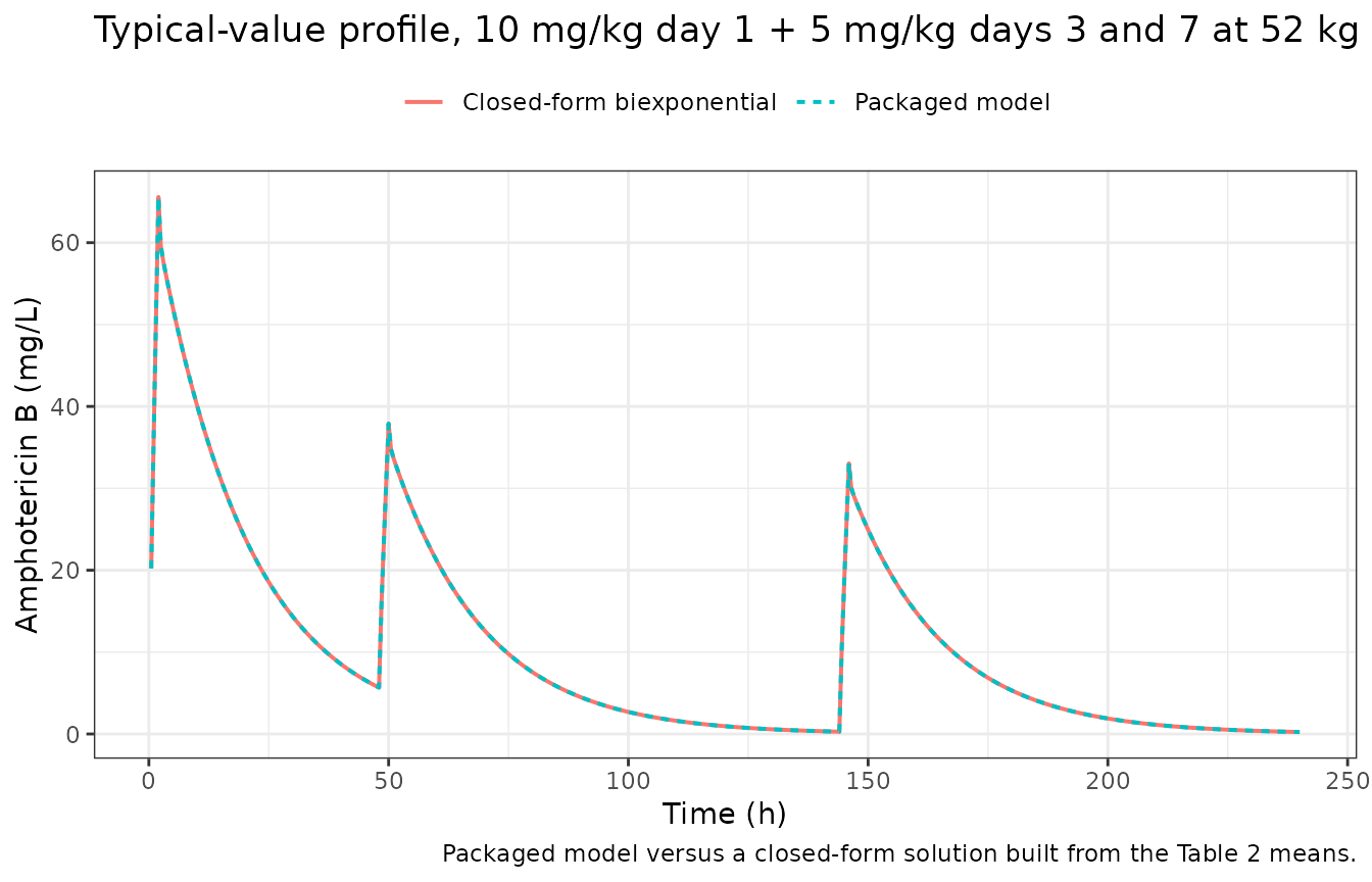

Mass balance and terminal half-life after a single 10 mg/kg dose

After a single dose, the area under the curve to infinity equals Dose / CL exactly, and the terminal half-life is log(2) / beta.

dose_single <- 10 * paper$wt_median
ev_single <- bind_rows(
  tibble(id = 1L, time = 0, evid = 1L, amt = dose_single, rate = dose_single / paper$tinf, cmt = "central"),
  tibble(id = 1L, time = seq(0, 336, by = 0.25), evid = 0L, amt = NA_real_, rate = NA_real_, cmt = "central")
) |>
  arrange(time, desc(evid))

sim_single <- rxode2::rxSolve(
  ui_typ,
  events = as.data.frame(ev_single),
  useLinCmt = FALSE,
  rtol = 1e-10, atol = 1e-12,
  returnType = "data.frame"
)
#> ℹ omega/sigma items treated as zero: 'etalcl', 'etalvc', 'etalk12', 'etalk21'
stopifnot("peripheral1" %in% names(sim_single))

ref_single <- biexp_conc(0, 0, dose_single, paper$tinf, paper$mean)
t_half_paper <- log(2) / ref_single$beta

auc_0_336 <- sum(diff(sim_single$time) * (head(sim_single$Cc, -1) + tail(sim_single$Cc, -1)) / 2)
auc_inf <- auc_0_336 + tail(sim_single$Cc, 1) / ref_single$beta
auc_closed <- dose_single / paper$mean[["cl"]]

late <- sim_single |> filter(time >= 120, time <= 240)
t_half_model <- log(2) / -coef(stats::lm(log(Cc) ~ time, data = late))[["time"]]

# Deterministic. The trapezoid on a 0.25 h grid is the only approximation in
# the AUC (realised error well under 0.1%); 1% still goes red on a wrong
# clearance or dose unit. The half-life fit is on a pure monoexponential tail.
stopifnot(
  abs(auc_inf - auc_closed) / auc_closed < 0.01,
  abs(t_half_model - t_half_paper) / t_half_paper < 0.01
)

tibble(
  Quantity = c(
    "Dose (mg)", "Dose / CL (mg*h/L)", "Simulated AUC0-inf (mg*h/L)",
    "alpha (1/h)", "beta (1/h)",
    "Terminal half-life, closed form (h)", "Terminal half-life, packaged model (h)"
  ),
  Value = c(dose_single, auc_closed, auc_inf, ref_single$alpha, ref_single$beta, t_half_paper, t_half_model)
) |>
  knitr::kable(digits = 3, caption = "Typical patient (52 kg) after a single 10 mg/kg 2 h infusion.")

Typical patient (52 kg) after a single 10 mg/kg 2 h infusion.

Quantity	Value
Dose (mg)	520.000
Dose / CL (mg*h/L)	1250.000
Simulated AUC0-inf (mg*h/L)	1250.000
alpha (1/h)	5.213
beta (1/h)	0.052
Terminal half-life, closed form (h)	13.438
Terminal half-life, packaged model (h)	13.438

Table 2 means versus medians

Table 2 reports both the mean and the median of every parameter’s nonparametric marginal distribution, and Methods says that “both mean and median parameter values were examined” without stating which set the final model’s population predictions used. The Abstract presents the means as the population estimates, so the means are encoded. The two sets differ by a factor of about ten on KCP and six on KPC, which is a direct sign that the NPAG distribution of the distribution rate constants is far from log-normal.

The Discussion states that “plasma concentrations fall to negligible levels 48-72 h after a single dose of 10 mg/kg”. Both parameter sets satisfy that statement, so it does not discriminate between them; the visible difference is in the first hours, where the medians’ slow distribution gives a peak almost twice as high.

mean_median <- bind_rows(
  tibble(set = "Table 2 means (encoded)", time = t_grid, Cc = biexp_conc(t_grid, 0, dose_single, paper$tinf, paper$mean)$conc),
  tibble(set = "Table 2 medians", time = t_grid, Cc = biexp_conc(t_grid, 0, dose_single, paper$tinf, paper$median)$conc)
)

neg <- mean_median |>
  group_by(set) |>
  summarise(
    cmax = max(Cc),
    c48 = Cc[time == 48],
    c72 = Cc[time == 72],
    .groups = "drop"
  ) |>
  mutate(pct72 = 100 * c72 / cmax)

# The Discussion's 'negligible by 48-72 h' claim: under 5% of the peak by 72 h
# for both parameter sets (realised 2.5% and 1.0%). Deterministic.
stopifnot(all(neg$pct72 < 5))

neg |>
  rename(
    "Parameter set" = set, "Cmax (mg/L)" = cmax, "C at 48 h (mg/L)" = c48,
    "C at 72 h (mg/L)" = c72, "C72 as % of Cmax" = pct72
  ) |>
  knitr::kable(digits = 2, caption = "Typical 52 kg patient after a single 10 mg/kg dose, closed form.")

Typical 52 kg patient after a single 10 mg/kg dose, closed form.

Parameter set	Cmax (mg/L)	C at 48 h (mg/L)	C at 72 h (mg/L)	C72 as % of Cmax
Table 2 means (encoded)	65.58	5.67	1.64	2.51
Table 2 medians	110.54	4.90	1.12	1.01

ggplot(mean_median |> filter(time > 0, time <= 168), aes(time, Cc, colour = set)) +
  geom_line(linewidth = 0.7) +
  geom_hline(yintercept = paper$lloq, linetype = "dashed") +
  scale_y_log10() +
  labs(
    x = "Time (h)", y = "Amphotericin B (mg/L)", colour = NULL,
    title = "Single 10 mg/kg dose at 52 kg: Table 2 means versus medians",
    caption = "Dashed line: assay LLOQ 0.25 mg/L."
  ) +
  theme_bw() +
  theme(legend.position = "top")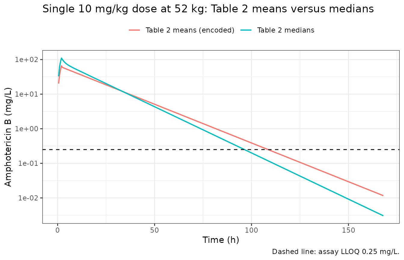

Virtual cohort

Original observed data are not publicly available. The cohort below reproduces the five AmBisome regimens of the two trials at 200 virtual patients per regimen. Weight drives only the mg/kg dose, since no covariate was retained; it is drawn from a log-normal matched to the Table 1 median and IQR.

# set.seed() seeds R's RNG, which draws the weights below. It does NOT seed
# rxode2's eta sampler, whose streams are partitioned per solver thread, so the
# drawn cohort differs between machines. Every assertion below holds for any
# cohort this model can produce.
set.seed(20221122)

n_arm <- 200L
wt_sdlog <- log(paper$wt_q3 / paper$wt_q1) / (2 * stats::qnorm(0.75))
cohort_wt <- pmin(pmax(stats::rlnorm(n_arm, log(paper$wt_median), wt_sdlog), 30), 100)

regimens <- list(
  "Phase II: 3 mg/kg/day x 14 days" = tibble(day = 1:14, mgkg = 3),
  "Phase II: 10 mg/kg day 1" = tibble(day = 1, mgkg = 10),
  "Phase II: 10 mg/kg day 1 + 5 mg/kg day 3" = tibble(day = c(1, 3), mgkg = c(10, 5)),
  "Phase II: 10 mg/kg day 1 + 5 mg/kg days 3, 7" = tibble(day = c(1, 3, 7), mgkg = c(10, 5, 5)),
  "Phase III: 10 mg/kg day 1" = tibble(day = 1, mgkg = 10)
)

make_arm <- function(i) {
  label <- names(regimens)[i]
  subj <- tibble(id = (i - 1L) * n_arm + seq_len(n_arm), WT = cohort_wt, treatment = label)
  dosing <- subj |>
    tidyr::crossing(regimens[[i]]) |>
    mutate(
      time = 24 * (day - 1), evid = 1L, amt = mgkg * WT,
      rate = amt / paper$tinf, cmt = "central"
    ) |>
    select(-day, -mgkg)
  obs <- subj |>
    tidyr::crossing(time = seq(0, 168, by = 1)) |>
    mutate(evid = 0L, amt = NA_real_, rate = NA_real_, cmt = "central")
  bind_rows(dosing, obs) |>
    arrange(id, time, desc(evid)) |>
    select(id, time, evid, amt, rate, cmt, WT, treatment)
}

events <- bind_rows(lapply(seq_along(regimens), make_arm))
stopifnot(!anyDuplicated(events[, c("id", "time", "evid")]))

sim <- rxode2::rxSolve(
  ui,
  events = as.data.frame(events),
  keep = c("WT", "treatment"),
  useLinCmt = FALSE,
  returnType = "data.frame"
) |>
  mutate(treatment = factor(treatment, levels = names(regimens)))

stopifnot(
  dplyr::n_distinct(sim$id) == length(regimens) * n_arm,
  !anyNA(sim$Cc),
  all(sim$Cc >= -1e-6 * max(sim$Cc))
)

Replicate published figures

Stott 2022 publishes only goodness-of-fit plots (Figure 1: observed versus population and individual predicted concentrations, regression r^2 0.52 and 0.90), which cannot be reproduced without the observed data. The simulated concentration-time profiles below are therefore companions rather than replications.

sim |>
  filter(time > 0) |>
  group_by(treatment, time) |>
  summarise(
    Q05 = quantile(Cc, 0.05),
    Q50 = quantile(Cc, 0.50),
    Q95 = quantile(Cc, 0.95),
    .groups = "drop"
  ) |>
  ggplot(aes(time)) +
  geom_ribbon(aes(ymin = Q05, ymax = Q95), alpha = 0.2) +
  geom_line(aes(y = Q50), linewidth = 0.6) +
  geom_hline(yintercept = paper$lloq, linetype = "dashed") +
  facet_wrap(~treatment, ncol = 2) +
  scale_y_log10() +
  coord_cartesian(ylim = c(0.01, NA)) +
  labs(
    x = "Time (h)", y = "Amphotericin B (mg/L)",
    title = "Simulated median and 90% interval by regimen",
    caption = "Dashed line: assay LLOQ 0.25 mg/L. Values below 0.01 mg/L are not drawn."
  ) +
  theme_bw()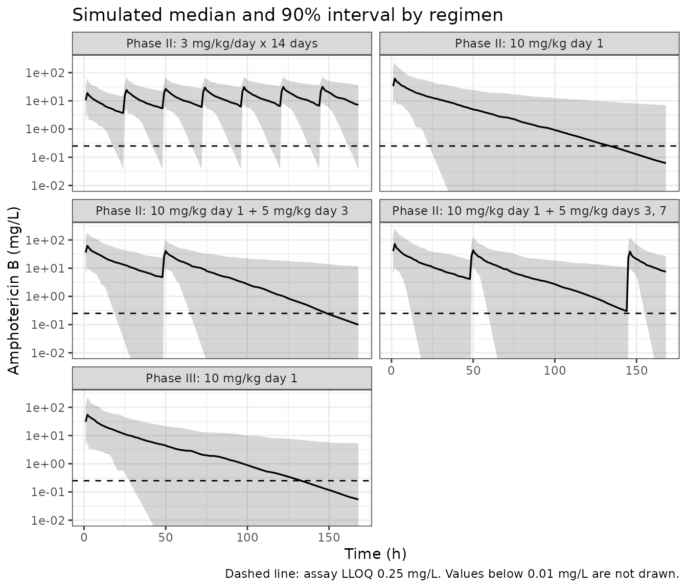

PKNCA validation

Stott 2022 computed AUC0-24, AUC0-168 and the first-week Cmax from Bayesian posterior predictions for its exposure-toxicity analysis, but does not print their values, so there is no published NCA to compare against. The block below reports the same metrics for the simulated cohort and checks the single-dose arms against the per-subject identity AUC0-inf = Dose / CL.

sim_nca <- sim |>
  filter(!is.na(Cc)) |>
  mutate(Cc = pmax(Cc, 0)) |>
  select(id, time, Cc, treatment)

# Guarantee a time = 0 row per subject; pre-dose concentration is zero.
sim_nca <- bind_rows(
  sim_nca,
  sim_nca |> distinct(id, treatment) |> mutate(time = 0, Cc = 0)
) |>
  distinct(id, treatment, time, .keep_all = TRUE) |>
  arrange(id, treatment, time)

conc_obj <- PKNCA::PKNCAconc(
  as.data.frame(sim_nca),
  Cc ~ time | treatment + id,
  concu = "mg/L", timeu = "h"
)

dose_df <- events |>
  filter(evid == 1) |>
  select(id, time, amt, treatment)
dose_obj <- PKNCA::PKNCAdose(as.data.frame(dose_df), amt ~ time | treatment + id, doseu = "mg")

intervals <- data.frame(
  start = 0,
  end = c(24, 168),
  auclast = TRUE,
  cmax = c(FALSE, TRUE),
  tmax = c(FALSE, TRUE)
)

nca_res <- PKNCA::pk.nca(PKNCA::PKNCAdata(conc_obj, dose_obj, intervals = intervals))

nca_res$result |>
  filter(PPTESTCD %in% c("auclast", "cmax", "tmax")) |>
  mutate(PPTESTCD = ifelse(PPTESTCD == "auclast", paste0("auc0-", end), PPTESTCD)) |>
  group_by(treatment, PPTESTCD) |>
  summarise(
    median = median(PPORRES),
    q25 = quantile(PPORRES, 0.25),
    q75 = quantile(PPORRES, 0.75),
    .groups = "drop"
  ) |>
  rename(
    "Regimen" = treatment, "NCA parameter" = PPTESTCD,
    "Median" = median, "P25" = q25, "P75" = q75
  ) |>
  knitr::kable(digits = 2, caption = "Simulated NCA by regimen: AUC0-24 and AUC0-168 (mg*h/L), first-week Cmax (mg/L) and tmax (h).")

Simulated NCA by regimen: AUC0-24 and AUC0-168 (mg*h/L), first-week Cmax (mg/L) and tmax (h).

Regimen	NCA parameter	Median	P25	P75
Phase II: 10 mg/kg day 1	auc0-168	1163.76	721.49	1977.52
Phase II: 10 mg/kg day 1	auc0-24	651.60	425.63	1104.94
Phase II: 10 mg/kg day 1	cmax	61.68	29.54	106.55
Phase II: 10 mg/kg day 1	tmax	2.00	2.00	2.00
Phase II: 10 mg/kg day 1 + 5 mg/kg day 3	auc0-168	1658.98	1022.01	2896.76
Phase II: 10 mg/kg day 1 + 5 mg/kg day 3	auc0-24	666.86	433.10	1034.23
Phase II: 10 mg/kg day 1 + 5 mg/kg day 3	cmax	62.62	35.93	105.92
Phase II: 10 mg/kg day 1 + 5 mg/kg day 3	tmax	2.00	2.00	2.00
Phase II: 10 mg/kg day 1 + 5 mg/kg days 3, 7	auc0-168	2018.59	1275.64	3218.07
Phase II: 10 mg/kg day 1 + 5 mg/kg days 3, 7	auc0-24	648.49	379.96	1112.59
Phase II: 10 mg/kg day 1 + 5 mg/kg days 3, 7	cmax	72.39	33.58	131.96
Phase II: 10 mg/kg day 1 + 5 mg/kg days 3, 7	tmax	2.00	2.00	2.00
Phase II: 3 mg/kg/day x 14 days	auc0-168	2094.10	1225.28	3714.27
Phase II: 3 mg/kg/day x 14 days	auc0-24	205.53	123.08	328.41
Phase II: 3 mg/kg/day x 14 days	cmax	31.48	19.06	45.57
Phase II: 3 mg/kg/day x 14 days	tmax	146.00	146.00	146.00
Phase III: 10 mg/kg day 1	auc0-168	1063.99	695.53	1763.77
Phase III: 10 mg/kg day 1	auc0-24	614.98	383.02	1052.90
Phase III: 10 mg/kg day 1	cmax	54.24	26.17	96.17
Phase III: 10 mg/kg day 1	tmax	2.00	2.00	2.00

single_arms <- c("Phase II: 10 mg/kg day 1", "Phase III: 10 mg/kg day 1")

intervals_single <- data.frame(start = 0, end = Inf, aucinf.obs = TRUE, half.life = TRUE)
conc_single <- PKNCA::PKNCAconc(
  as.data.frame(sim_nca |> filter(treatment %in% single_arms)),
  Cc ~ time | treatment + id,
  concu = "mg/L", timeu = "h"
)
dose_single_obj <- PKNCA::PKNCAdose(
  as.data.frame(dose_df |> filter(treatment %in% single_arms)),
  amt ~ time | treatment + id,
  doseu = "mg"
)
nca_single <- PKNCA::pk.nca(PKNCA::PKNCAdata(conc_single, dose_single_obj, intervals = intervals_single))

chk <- nca_single$result |>
  filter(PPTESTCD == "aucinf.obs") |>
  select(id, aucinf = PPORRES) |>
  inner_join(
    sim |> distinct(id, cl, treatment),
    by = "id"
  ) |>
  inner_join(dose_df |> select(id, amt), by = "id") |>
  mutate(pct_diff = 100 * (aucinf - amt / cl) / (amt / cl)) |>
  filter(!is.na(pct_diff))

# AUC0-inf from PKNCA against each subject's own Dose / CL. The two sides use
# the same drawn parameters, so the centre is numerical error only; the tail
# carries the extrapolation error of subjects whose sampled k21 is small enough
# that the 168 h window does not reach the terminal phase.
stopifnot(
  nrow(chk) > 0.9 * length(single_arms) * n_arm,
  abs(median(chk$pct_diff)) < 2,
  quantile(abs(chk$pct_diff), 0.9) < 10
)

chk |>
  group_by(treatment) |>
  summarise(
    "Subjects" = n(),
    "Median AUC0-inf (mg*h/L)" = median(aucinf),
    "Median Dose/CL (mg*h/L)" = median(amt / cl),
    "Median % difference" = median(pct_diff),
    "90th percentile |% difference|" = quantile(abs(pct_diff), 0.9),
    .groups = "drop"
  ) |>
  rename("Regimen" = treatment) |>
  knitr::kable(digits = 2, caption = "Single-dose arms: PKNCA AUC0-inf against each subject's Dose / CL.")

Single-dose arms: PKNCA AUC0-inf against each subject’s Dose / CL.

Regimen	Subjects	Median AUC0-inf (mg*h/L)	Median Dose/CL (mg*h/L)	Median % difference	90th percentile |% difference|
Phase II: 10 mg/kg day 1	200	1371.41	1372.67	-0.03	0.32
Phase III: 10 mg/kg day 1	200	1203.19	1203.43	-0.02	0.29

Assumptions and deviations

• Nonparametric distributions approximated as log-normal. Pmetrics NPAG estimates a discrete joint distribution over support points and Stott 2022 publishes only each marginal’s mean, median and SD (Table 2). Each parameter is encoded as a log-normal whose median is the reported mean and whose variance is log(1 + (SD / mean)^2) (CVs of 87, 99, 151 and 138% for clearance, volume, KCP and KPC). No correlations are published, so the etas are independent. The nonparametric shape cannot be reproduced: for a log-normal the mean-to-median ratio is exp(omega^2 / 2), which is 1.33 and 1.41 for clearance and volume against the reported 1.21 and 1.23, and 1.81 and 1.70 for KCP and KPC against the reported 10.2 and 6.1. Simulated distribution-phase behaviour is therefore the least reliable part of the stochastic model.

• Means used as the typical values. Methods says both mean and median parameter values were examined, without stating which the final model’s population predictions used; the Abstract reports the means as the “population PK parameter estimates”. The means are encoded, as in the same group’s amphotericin B deoxycholate model (Stott_2018_amphotericinB_deoxycholate), and the medians are compared above. The Discussion’s single-dose washout statement holds for either set.

• Residual error is an assay-precision stand-in, not a fitted estimate. Results states that additive error (the Pmetrics lambda term, combined in quadrature with the assay error polynomial) was selected, but neither the assay polynomial nor the fitted lambda is printed. addSd (lambda) is therefore fixed to 0 and propSd to the reported assay coefficient of variation of 9% (Materials and methods: “The coefficient of variation was <9.0% over the concentration range 0.25-50.0 mg/L”). The encoded residual understates the observation scatter. Every check in this vignette is run on Cc, the individual prediction, so none depends on it.

• No covariates. Age, sex, weight, baseline serum creatinine and CD4+ count were screened by stepwise multivariate linear regression on the Bayesian posterior parameters and none was retained. They are recorded in the model file’s covariatesDataExcluded metadata. Weight enters the simulation only through the mg/kg dose.

• Typographical errors in the source. Table 1 gives serum creatinine in “mmol/L”; a median of 64.0 is only possible in umol/L, the unit the Toxicity section uses. Results describes the Figure 1 regression as being of “observed-versus-predicted concentrations of DAmB”, where the analyte is liposomal amphotericin B. Neither affects a model value.

• Simulated weights. Table 1 reports the weight median and IQR only; the virtual cohort draws a log-normal with median 52.0 kg and the IQR-matched log-SD, truncated to 30-100 kg.

• Exposure-toxicity and meta-analysis layers not extracted. The exposure-toxicity logistic regressions report only odds ratios of 1.0 per unit AUC (Table 3) with no intercepts, and the random-effects meta-analysis of AmBisome monotherapy outcomes reports only residual heterogeneity (tau^2 0.0023 falling to 0.0003 with moderators) and P values, not the moderator coefficients. Neither can be encoded from the printed values.

• Errata. No erratum or correction was found for this article (Europe PMC search, October 2026).