Morphine and M6G brain PBPK (Verscheijden 2021) • nlmixr2lib

Model and source

Citation: Verscheijden LFM, Litjens CHC, Koenderink JB, Mathijssen RHJ, Verbeek MM, de Wildt SN, Russel FGM. Physiologically based pharmacokinetic/pharmacodynamic model for the prediction of morphine brain disposition and analgesia in adults and children. PLoS Comput Biol. 2021;17(3):e1008786. doi:10.1371/journal.pcbi.1008786. Adult and paediatric physiology (S1 Table) and brain framework: Verscheijden LFM, Koenderink JB, de Wildt SN, Russel FGM. Development of a physiologically-based pharmacokinetic pediatric brain model for prediction of cerebrospinal fluid drug concentrations and the influence of meningitis. PLoS Comput Biol. 2019;15(6):e1007117. doi:10.1371/journal.pcbi.1007117.
Description: PBPK/PD (whole-body, permeability-limited 4-compartment brain, R/deSolve). Morphine and its active metabolite morphine-6-glucuronide (M6G) in adults, children and neonates (Verscheijden et al. 2021, PLoS Comput Biol). Thirteen perfusion-limited body compartments per analyte (venous and arterial blood, lung, adipose, bone, heart, kidney, muscle, skin, spleen, gut, liver, rest of body) with Rodgers and Rowland tissue partition coefficients computed from age-dependent tissue composition, plus the Gaohua / Verscheijden brain model (brain blood, brain mass, cranial CSF, spinal CSF) with passive blood-brain and blood-CSF barrier permeability and active P-glycoprotein efflux of morphine from brain mass, scaled from MDCKII-Pgp transwell data by in vitro-in vivo extrapolation. Organ volumes, blood flows, haematocrit and CSF flows are age-, sex-, weight- and height-dependent (paediatric equations below 18 y, adult equations of Verscheijden 2019 from 18 y). Morphine is cleared from venous blood; a fixed fraction of the cleared mass (corrected for molecular weight) is formed as M6G. The PD part converts unbound brain-mass morphine and M6G into competitive mu-opioid receptor occupancy and a sigmoid relative analgesic response. Forward-simulation model: all parameters are fixed; IIV reproduces the virtual-population variability of the deposited code; no residual error was reported.
Article: https://doi.org/10.1371/journal.pcbi.1008786 (open access)
Deposited code: S1 File of the article, the complete deSolve implementation of the paediatric model (2.6-16.4 y version).
Structural brain framework and adult physiology: https://doi.org/10.1371/journal.pcbi.1007117 (Verscheijden et al. 2019, S1 Table, adult column).

Verscheijden et al. built a whole-body physiologically based pharmacokinetic (PBPK) model for morphine and its active metabolite morphine-6-glucuronide (M6G), with a four-compartment brain (brain blood, brain mass, cranial CSF, spinal CSF). Passive blood-brain and blood-CSF barrier permeability came from a rat perfusion study, and active P-glycoprotein (Pgp) efflux of morphine was scaled from MDCKII-Pgp transwell experiments by in vitro-in vivo extrapolation (IVIVE), with postnatal Pgp maturation. Organ volumes, flows and tissue composition depend on age, sex, weight and height, so one model file covers neonates, children and adults. A receptor-occupancy module converts unbound brain-mass concentrations of morphine and M6G into a relative response.

This vignette validates the pharmacokinetic part of the model: the IVIVE clearance, the mass balance, the volume of distribution, the published with/without-Pgp brain exposure ratio, and the concentration-time profiles of the paper’s verification scenarios. The receptor-occupancy output is shown only as its relative-response curve.

Model structure

 venous blood --> lung --> arterial blood --> 10 perfused tissues --> venous blood
      |  CL (blood)                |
      v                            +--> brain blood <--PSb, Pgp--> brain mass
  0.1 x CL x MW ratio                     ^   PSc        PSe  |  bulk flow
  forms M6G (venous)                      +--> cranial CSF <--+
                                                    ^ |
                                         spinal CSF -+ +- sink flows to blood

17 amount states for morphine (venous, arterial, lung, adipose, bone, heart, kidney, muscle, skin, spleen, other, gut, liver, brain_vascular, brain, brain_csf_sas_cranial, brain_csf_sas_spinal) and the same 17 with an _m6g suffix for M6G.
IV doses go into venous. Clearance acts on the venous blood concentration; a molecular-weight-corrected fraction of the cleared morphine appears as M6G in venous blood.
Outputs: Cc (plasma morphine), Cc_m6g, Cbrain_u (unbound brain mass, the paper’s surrogate for microdialysis ECF), Ccsf (cranial CSF), Ccsf_spinal and the M6G equivalents, plus effect_rel (relative response).

Population

The paper fits no parameter to individual data. Drug inputs come from the literature and the authors’ own MDCKII-Pgp experiments (Table 1), and 11 published studies plus 19 neonatal CSF biobank samples were used only for verification (Table 2):

Adults 19-69 y: neurological / neurosurgical patients after 0.38 mg/kg IV (Meineke 2002; plasma and ventricular CSF), and traumatic brain injury patients after 10 mg IV (Bouw 2001, Ederoth 2003; plasma and microdialysis ECF).
Children 1-18 y with acute leukaemia after 0.25 mg/kg IV (Hain 1999; plasma and lumbar CSF), and three children 3.5-9.5 y on a 0.03 mg/kg/h infusion (Ketharanathan 2019; plasma and ECF).
Neonates after 0.1 mg/kg IV at 1.1 and 29 days postnatal age (Pokela 1993).

The paper simulated 500 virtual individuals per scenario, matched to each study’s age range, dose and sex ratio. The population metadata of the model file records these facts.

str(readModelDb("Verscheijden_2021_morphine_pbpk")()$population)
#> List of 10
#>  $ species       : chr "human"
#>  $ n_subjects    : int NA
#>  $ n_studies     : int 11
#>  $ age_range     : chr "10 days to 69 years (neonates, children 1-18 y, adults 18-69 y)"
#>  $ weight_range  : chr "not reported; generated from age and height in the virtual populations"
#>  $ sex_female_pct: num NA
#>  $ disease_state : chr "Mixed. PK verification: neurological / neurosurgical patients (Meineke 2002), traumatic brain injury (Bouw 2001"| __truncated__
#>  $ dose_range    : chr "Single IV morphine 0.025-0.38 mg/kg or 10-28 mg; continuous IV infusion 0.03 mg/kg/h (children) and 0.25 mg/kg/h for 1 h."
#>  $ regions       : chr "Europe (Netherlands, Germany, Sweden, UK, Austria)"
#>  $ notes         : chr "Forward-simulation PBPK/PD: no parameter was estimated from individual data in this paper. Drug-specific inputs"| __truncated__

Source trace

Model element	Value	Source
Morphine CL, adults	1.962 L/h/kg	Table 1, CLiv (adult)
Morphine CL, children and neonates	60 x 1.62 x (WT/70)^(1.47 - 0.59 WT^4.62/(4.014.62 + WT^4.62)) L/h	Table 1, CLiv (2-18y), (neonates); S1 File line 706
M6G CL, adults / children / neonates	0.131 / 0.114 / 0.017 L/h/kg	Table 1, CLiv M6G
Fraction of CL forming M6G	0.1 (2 y to adult), 0.044 (neonates)	Table 1
MW morphine / M6G	285.343 / 461.467 g/mol	Table 1
LogP, pKa, EP morphine	0.89, 8.21 (base), 1.34	Table 1
LogP, pKa, EP M6G	-2.9, 2.87 (acid) / 9.12 (base), 0.15	Table 1
Olive oil:water logP morphine / M6G	-0.35765 / -4.5835	S1 File lines 572, 591
M6G Kp scalar	0.5	Methods; S1 File line 599
fu plasma / brain mass / CSF, morphine	0.64 / 0.5 / 1	Table 1
fu plasma / brain mass / CSF, M6G	0.83 / 0.99 / 1	Table 1
fu blood morphine	0.64 / 1.14	S1 File line 475
PSb morphine / M6G	0.2112 / 0.0072 L/h per kg brain	Table 1
PSc	0.5 x PSb	Table 1
PSe	300 L/h	Table 1
Pgp IVIVE inputs	ER 1.30, Papp 2.12e-6 cm/s, SA 0.33 cm^2, 81.4 ug protein, 4.21 / 0.19 pmol/mg, 0.244 mg/g, 1400 g	Table 1; Methods Eqs 2-3
Pgp maturation	41% at term, 100% at 6 months	Methods
CSF production adult / child / neonate	0.021 / 0.024 / 0.010 L/h	2019 S1 Table; Methods
Bulk flow, spinal sink and outflow fractions	0.25, 0.38, 0.9	2019 S1 Table; S1 File lines 403-411
Adult haematocrit male / female	0.43 / 0.38	2019 S1 Table
Paediatric organ volumes, flows, haematocrit, tissue composition	equations	S1 File lines 266-569
Adult organ volumes, flows, tissue composition	equations	2019 S1 Table, adult column
Rodgers and Rowland Kp (base; zwitterion for M6G)	equations	S1 File lines 571-610
Morphine and M6G ODEs	equations	S1 File lines 91-128
Receptor occupancy and response	KM 11.8 / 42.5 nM, BR50 59.26 / 17, Hill 4.217 / 2.2	Methods Eqs 4-6; S1 File lines 964-983
IIV (SD of log-normal draws)	CL 0.4, M6G CL 0.18, CSF production 0.1, bulk 0.08, sink 0.3, outflow 1, haematocrit 0.065 / 0.071	S1 File lines 400-492, 707-711

Virtual cohorts

Paediatric height and weight are generated with the sex-specific age-to-height and height-to-weight equations of the deposited code (S1 File lines 14-38), including their log-normal variability. The deposited code has no adult generator, so adult height and weight are drawn from normal and log-normal distributions with typical European values (see Assumptions). Each arm has 100 subjects (50% female).

paed_height <- function(age, female) {
  male_h <- 0.0000176179 * age^7 - 0.00119874 * age^6 + 0.0323848 * age^5 -
    0.444112 * age^4 + 3.2946 * age^3 - 13.2191 * age^2 + 33.75 * age + 52.62152
  fem_h <- -0.00000151027 * age^8 + 0.000121261 * age^7 - 0.0040023 * age^6 +
    0.070179 * age^5 - 0.708233 * age^4 + 4.1872 * age^3 - 14.3393 * age^2 +
    33.84778 * age + 51.535477
  ifelse(female == 1, fem_h * exp(rnorm(length(age), 0, 0.052)), male_h * exp(rnorm(length(age), 0, 0.057)))
}

paed_weight <- function(age, height, female) {
  male_w <- 7.826 * (1 - exp(age * -1.2)) + exp(height * 0.0209 + 0.023 * age)
  fem_w <- 5.454 * (1 - exp(age * -1.57)) + exp(height * 0.0224 + 0.019 * age)
  ifelse(female == 1, fem_w * exp(rnorm(length(age), 0, 0.10)), male_w * exp(rnorm(length(age), 0, 0.15)))
}

make_cohort <- function(n, age_lo, age_hi, arm, id0 = 0) {
  female <- rep(c(0, 1), length.out = n)
  age <- runif(n, age_lo, age_hi)
  if (age_lo >= 18) {
    ht <- ifelse(female == 1, rnorm(n, 165, 7), rnorm(n, 178, 7))
    wt <- ifelse(female == 1, 66, 80) * exp(rnorm(n, 0, 0.15))
  } else {
    ht <- paed_height(age, female)
    wt <- paed_weight(age, ht, female)
  }
  data.frame(id = id0 + seq_len(n), arm = arm, AGE = age, WT = wt, HT = ht, SEXF = female)
}

# One dosing record per subject plus an observation grid on the venous state.
# dur = 0 gives an IV bolus; dur > 0 a constant-rate infusion.
make_events <- function(cohort, dose_mg, dur, obs_times) {
  dose <- cohort |>
    mutate(time = 0, amt = dose_mg, rate = if (dur > 0) dose_mg / dur else 0, evid = 1L, cmt = "venous")
  obs <- tidyr::crossing(cohort, time = obs_times) |>
    mutate(amt = 0, rate = 0, evid = 0L, cmt = "venous")
  bind_rows(dose, obs) |> arrange(id, time, desc(evid))
}

rxode2::rxSetSeed(20210304)
set.seed(20210304)
n_arm <- 100
obs_24 <- sort(unique(c(seq(0, 0.5, by = 0.0125), seq(0.5, 2, by = 0.1), seq(2.25, 24, by = 0.25))))
# "Single IV dose": a 5-min infusion into venous blood (see Assumptions)
iv_dur <- 5 / 60

coh_adult <- make_cohort(n_arm, 19, 69, "Adults 0.38 mg/kg (Fig 1A)")
coh_paed <- make_cohort(n_arm, 1.4, 15.9, "Children 0.25 mg/kg (Fig 1B)", id0 = 1000)
coh_adult_ecf <- make_cohort(n_arm, 32, 52, "Adults 10 mg (Fig 2A)", id0 = 2000)
coh_paed_ecf <- make_cohort(n_arm, 3.5, 9.5, "Children 0.03 mg/kg/h (Fig 2A)", id0 = 3000)

ev <- bind_rows(
  make_events(coh_adult, 0.38 * coh_adult$WT, iv_dur, obs_24),
  make_events(coh_paed, 0.25 * coh_paed$WT, iv_dur, obs_24),
  make_events(coh_adult_ecf, 10, iv_dur, obs_24),
  # continuous infusion over the whole 24-h window
  make_events(coh_paed_ecf, 0.03 * coh_paed_ecf$WT * 24, 24, obs_24)
)

bind_rows(coh_adult, coh_paed, coh_adult_ecf, coh_paed_ecf) |>
  group_by(arm) |>
  summarise(
    n = n(), `female (%)` = 100 * mean(SEXF),
    `age (y)` = sprintf("%.1f (%.1f-%.1f)", median(AGE), min(AGE), max(AGE)),
    `weight (kg)` = sprintf("%.1f (%.1f-%.1f)", median(WT), min(WT), max(WT)),
    `height (cm)` = sprintf("%.0f (%.0f-%.0f)", median(HT), min(HT), max(HT)),
    .groups = "drop"
  ) |>
  knitr::kable(caption = "Virtual cohorts: median (range).")

Virtual cohorts: median (range).
arm	n	female (%)	age (y)	weight (kg)	height (cm)
Adults 0.38 mg/kg (Fig 1A)	100	50	45.3 (19.3-68.1)	74.2 (50.1-125.7)	173 (151-198)
Adults 10 mg (Fig 2A)	100	50	41.6 (32.3-52.0)	72.6 (46.6-123.1)	172 (143-188)
Children 0.03 mg/kg/h (Fig 2A)	100	50	6.7 (3.6-9.2)	23.0 (12.9-39.2)	121 (94-143)
Children 0.25 mg/kg (Fig 1B)	100	50	9.4 (1.7-15.8)	29.1 (11.4-79.7)	133 (83-182)

Simulation

mod <- readModelDb("Verscheijden_2021_morphine_pbpk")
keep_cols <- c("Cc", "Cc_m6g", "Cbrain_u", "Ccsf", "Ccsf_spinal", "Cbrain_u_m6g", "Ccsf_m6g", "Ccsf_spinal_m6g")
sim <- rxode2::rxSolve(mod, ev, keep = "arm", returnType = "data.frame") |>
  select(id, time, arm, all_of(keep_cols), cl, bp)
#> ℹ parameter labels from comments will be replaced by 'label()'

summ <- sim |>
  pivot_longer(all_of(keep_cols), names_to = "output", values_to = "conc") |>
  group_by(arm, output, time) |>
  summarise(
    median = median(conc), lo = quantile(conc, 0.05), hi = quantile(conc, 0.95),
    .groups = "drop"
  )

plot_band <- function(d, title) {
  ggplot(d, aes(time, median)) +
    geom_ribbon(aes(ymin = lo, ymax = hi), fill = "grey80") +
    geom_line() +
    facet_wrap(~panel, scales = "free_y") +
    scale_y_log10() +
    labs(x = "Time (h)", y = "Concentration (mg/L)", title = title,
         caption = "Line: median; band: 90% interval of the virtual cohort.")
}

panel_labels <- c(
  Cc = "Plasma morphine", Cc_m6g = "Plasma M6G",
  Ccsf = "Cranial CSF morphine", Ccsf_m6g = "Cranial CSF M6G",
  Ccsf_spinal = "Spinal CSF morphine", Ccsf_spinal_m6g = "Spinal CSF M6G",
  Cbrain_u = "Unbound brain (ECF) morphine"
)

Replicate published figures

Figure 1A – adults, plasma and ventricular CSF

summ |>
  filter(arm == "Adults 0.38 mg/kg (Fig 1A)", output %in% c("Cc", "Cc_m6g", "Ccsf", "Ccsf_m6g"), time > 0) |>
  mutate(panel = factor(panel_labels[output], levels = panel_labels[c("Cc", "Cc_m6g", "Ccsf", "Ccsf_m6g")])) |>
  plot_band("Adults, 0.38 mg/kg IV")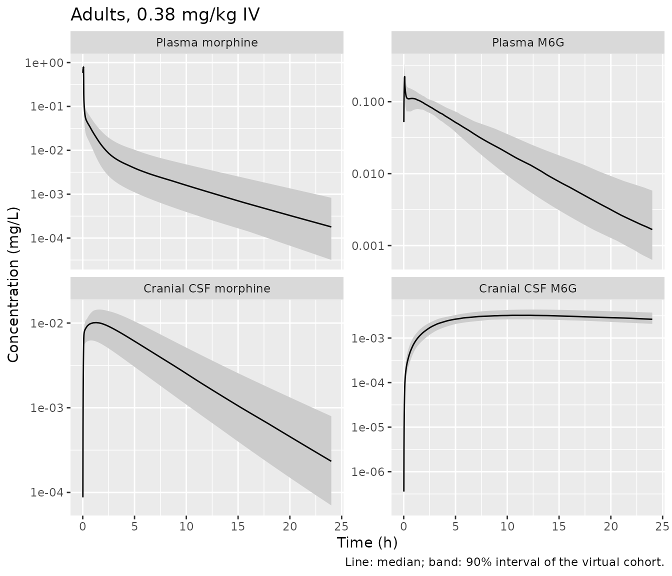

Replicates Figure 1A of Verscheijden 2021. The ventricular-drain samples are compared with the cranial CSF compartment.

Figure 1B – children, plasma and lumbar CSF

summ |>
  filter(arm == "Children 0.25 mg/kg (Fig 1B)", output %in% c("Cc", "Cc_m6g", "Ccsf_spinal", "Ccsf_spinal_m6g"), time > 0) |>
  mutate(panel = factor(panel_labels[output], levels = panel_labels[c("Cc", "Cc_m6g", "Ccsf_spinal", "Ccsf_spinal_m6g")])) |>
  plot_band("Children 1.4-15.9 y, 0.25 mg/kg IV")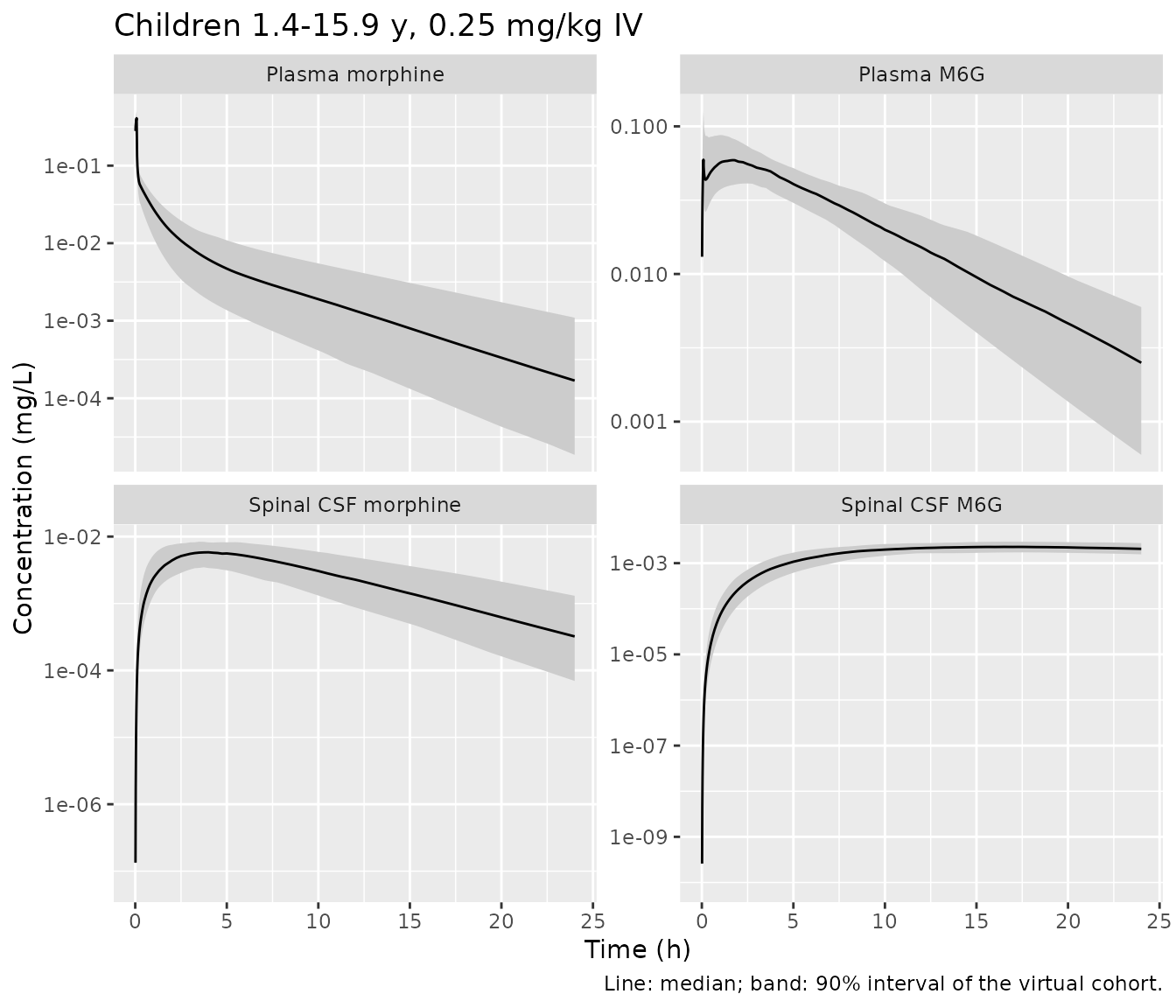

Replicates Figure 1B of Verscheijden 2021. Lumbar-puncture samples are compared with the spinal CSF compartment.

Figure 2A – plasma and brain ECF

summ |>
  filter(grepl("Fig 2A", arm), output %in% c("Cc", "Cbrain_u"), time > 0) |>
  mutate(panel = paste(panel_labels[output], "|", sub(" \\(Fig 2A\\)", "", arm))) |>
  plot_band("Plasma and unbound brain (ECF) morphine")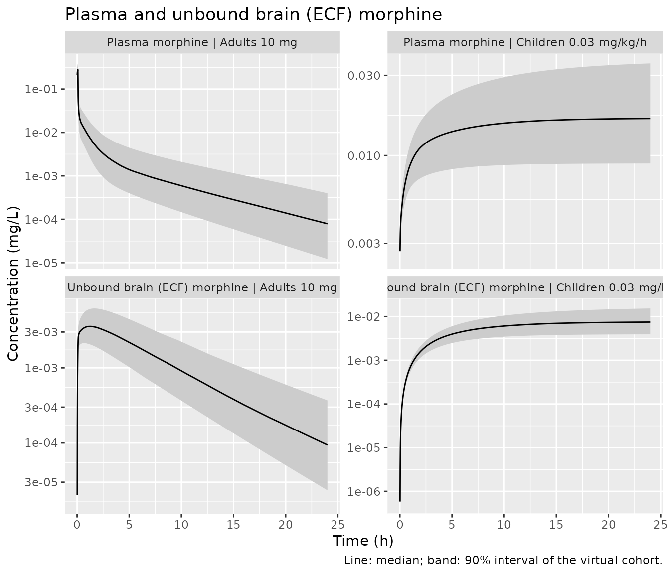

Replicates Figure 2A of Verscheijden 2021. As in the paper, the unbound brain-mass concentration stands in for the microdialysis ECF measurement. The paediatric infusion reaches a brain plateau within the first day, while the plasma profile is flat from the first hours; the paper notes that one measured 9.5-year-old needed more than 20 h to reach ECF equilibrium.

Figure 2B – neonatal plasma

neo <- data.frame(
  id = 1:2, arm = c("1.1 days postnatal", "29 days postnatal"),
  AGE = c(1.1, 29) / 365.25, SEXF = 0
)
neo$HT <- 52.62152 + 33.75 * neo$AGE # deposited male height polynomial near birth
neo$WT <- 7.826 * (1 - exp(neo$AGE * -1.2)) + exp(neo$HT * 0.0209 + 0.023 * neo$AGE)
ev_neo <- make_events(neo, 0.1 * neo$WT, iv_dur, obs_24)
# Typical-value solves, one subject at a time
solve_each <- function(m, events) {
  bind_rows(lapply(split(events, events$id), function(e) {
    rxode2::rxSolve(m, e, keep = "arm", returnType = "data.frame") |> mutate(id = e$id[1])
  }))
}
sim_neo <- solve_each(rxode2::zeroRe(mod), ev_neo)
#> ℹ parameter labels from comments will be replaced by 'label()'
#> ℹ omega/sigma items treated as zero: 'etalcl', 'etalcl_m6g', 'etalq_csf_prod', 'etalf_bulk', 'etalf_ssink', 'etalf_sout', 'etalhct'
#> ℹ omega/sigma items treated as zero: 'etalcl', 'etalcl_m6g', 'etalq_csf_prod', 'etalf_bulk', 'etalf_ssink', 'etalf_sout', 'etalhct'

ggplot(filter(sim_neo, time > 0), aes(time, Cc, colour = arm)) +
  geom_line() +
  scale_y_log10() +
  labs(x = "Time (h)", y = "Plasma morphine (mg/L)", colour = NULL,
       title = "Typical neonates, 0.1 mg/kg IV")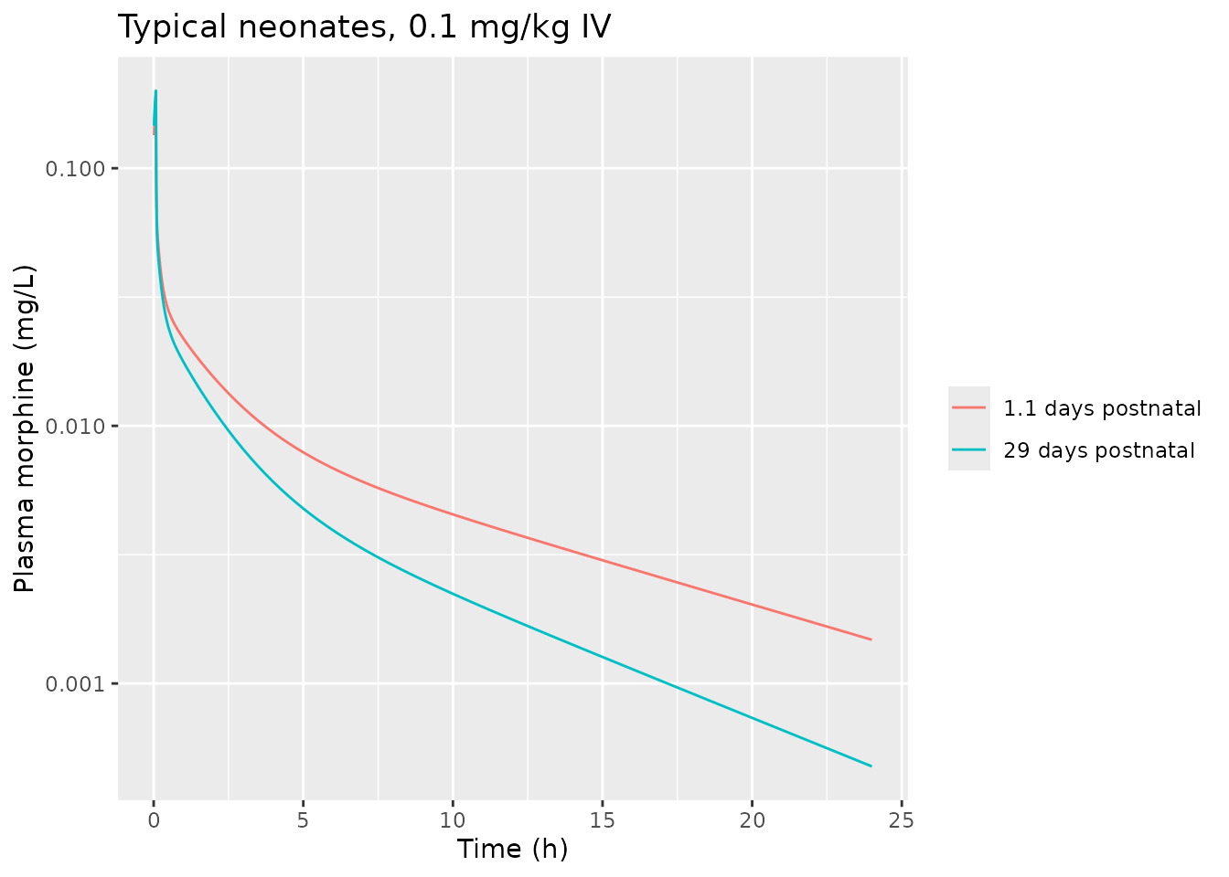

Replicates Figure 2B of Verscheijden 2021 (typical-value profiles). Neonatal clearance uses the bodyweight-dependent-exponent equation, and M6G formation falls to 4.4% of clearance in neonates.

Figure 2D – Pgp contribution to brain exposure

The paper reports that adding Pgp efflux lowers adult brain ECF exposure 1.3-fold (AUC without Pgp / AUC with Pgp = 1.3) after 0.38 mg/kg. Pgp is removed by setting the net in vitro efflux ratio to 1, which makes the IVIVE efflux clearance zero.

typ_adult <- data.frame(id = 1, arm = "typical adult", AGE = 40, WT = 70, HT = 176, SEXF = 0)
obs_48 <- seq(0, 48, by = 0.05)
ev_typ <- make_events(typ_adult, 0.38 * 70, iv_dur, obs_48)
mod_typ <- rxode2::zeroRe(mod)
#> ℹ parameter labels from comments will be replaced by 'label()'
mod_nopgp <- mod_typ |> rxode2::ini(er_pgp = 1)
#> ℹ change initial estimate of `er_pgp` to `1`

s_pgp <- rxode2::rxSolve(mod_typ, ev_typ, returnType = "data.frame")
#> ℹ omega/sigma items treated as zero: 'etalcl', 'etalcl_m6g', 'etalq_csf_prod', 'etalf_bulk', 'etalf_ssink', 'etalf_sout', 'etalhct'
s_nopgp <- rxode2::rxSolve(mod_nopgp, ev_typ, returnType = "data.frame")
#> ℹ omega/sigma items treated as zero: 'etalcl', 'etalcl_m6g', 'etalq_csf_prod', 'etalf_bulk', 'etalf_ssink', 'etalf_sout', 'etalhct'

trap <- function(t, y) sum(diff(t) * (head(y, -1) + tail(y, -1)) / 2)
auc_ratio <- trap(s_nopgp$time, s_nopgp$Cbrain_u) / trap(s_pgp$time, s_pgp$Cbrain_u)

bind_rows(
  mutate(s_pgp, scenario = "Pgp included"),
  mutate(s_nopgp, scenario = "Pgp not included")
) |>
  filter(time > 0, time <= 24) |>
  ggplot(aes(time, Cbrain_u, colour = scenario)) +
  geom_line() +
  scale_colour_manual(values = c("Pgp included" = "red", "Pgp not included" = "black")) +
  labs(x = "Time (h)", y = "Unbound brain (ECF) morphine (mg/L)", colour = NULL,
       title = sprintf("Typical adult, 0.38 mg/kg IV: AUC ratio = %.3f (paper: 1.3)", auc_ratio))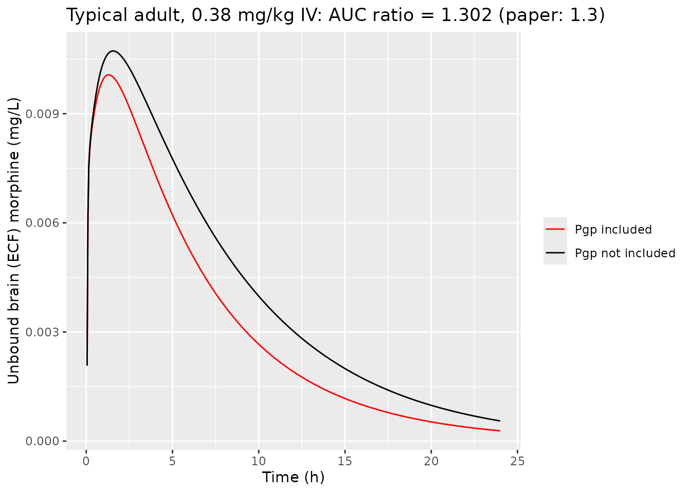


stopifnot(abs(auc_ratio - 1.3) < 0.05)

Replicates Figure 2D of Verscheijden 2021. Both curves use the same typical parameters, so the ratio is deterministic.

Clearance placement

The deposited S1 File removes the cleared morphine from the arterial compartment while computing it from the venous concentration (S1 File line 97, -(CL_iv * Cblv) in dCbla). The 2019 framework code removes it from venous blood (2019 S1 File line 81). The two forms clear the same mass, but the arterial form lowers the concentration reaching the tissues and the brain. The model file uses the venous form. Below, the deposited form is rebuilt by swapping the four blood ODEs, and both are compared with values digitised by the maintainers from the paper’s own figures:

Figure 2D, typical adult after 0.38 mg/kg with Pgp: unbound brain (ECF) morphine of 11.4, 11.8, 11.1, 8.2, 3.4, 1.4 and 0.59 ng/mL at 1, 2, 3, 5, 10, 15 and 20 h.
Figure 2A, 9.5-year-old on 0.03 mg/kg/h: median plateaus of about 26 ng/mL (plasma) and 12.2 ng/mL (ECF), an ECF:plasma ratio of 0.47. The ratio is used because the child’s individual weight and clearance are not reported.

mod_deposited <- rxode2::rxode2(mod_typ) |>
  rxode2::model(
    d/dt(venous) <- q_adipose * c_ad / kp_adipose * bp + q_bone * c_bo / kp_bone * bp +
      q_heart * c_he / kp_heart * bp + q_kidney * c_ki / kp_kidney * bp +
      q_muscle * c_mu / kp_muscle * bp + q_skin * c_sk / kp_skin * bp +
      q_liver * c_li / kp_liver * bp + q_brain * c_bb + q_rest * c_ot * bp - q_lung * c_ven,
    d/dt(arterial) <- q_lung * c_lung / kp_lung * bp -
      (q_rest + q_brain + q_adipose + q_bone + q_heart + q_kidney + q_muscle + q_skin + q_spleen + q_gut + q_ha) * c_art -
      cl * c_ven,
    d/dt(venous_m6g) <- cl * c_ven * f_form +
      q_adipose * m_ad / kp_adipose_m6g * bp_m6g + q_bone * m_bo / kp_bone_m6g * bp_m6g +
      q_heart * m_he / kp_heart_m6g * bp_m6g + q_kidney * m_ki / kp_kidney_m6g * bp_m6g +
      q_muscle * m_mu / kp_muscle_m6g * bp_m6g + q_skin * m_sk / kp_skin_m6g * bp_m6g +
      q_liver * m_li / kp_liver_m6g * bp_m6g + q_brain * m_bb + q_rest * m_ot / kp_other_m6g * bp_m6g -
      q_lung * m_ven,
    d/dt(arterial_m6g) <- q_lung * m_lung / kp_lung_m6g * bp_m6g -
      (q_rest + q_brain + q_adipose + q_bone + q_heart + q_kidney + q_muscle + q_skin + q_spleen + q_gut + q_ha) * m_art -
      cl_m6g * m_ven
  )

fig2d <- data.frame(
  time = c(1, 2, 3, 5, 10, 15, 20),
  digitised = c(11.4, 11.8, 11.1, 8.16, 3.44, 1.42, 0.589)
)
ecf_at <- function(m) {
  s <- rxode2::rxSolve(m, ev_typ, returnType = "data.frame")
  approx(s$time, s$Cbrain_u * 1000, fig2d$time)$y
}
fig2d$model <- ecf_at(mod_typ)
#> ℹ omega/sigma items treated as zero: 'etalcl', 'etalcl_m6g', 'etalq_csf_prod', 'etalf_bulk', 'etalf_ssink', 'etalf_sout', 'etalhct'
fig2d$deposited <- ecf_at(mod_deposited)
#> ℹ omega/sigma items treated as zero: 'etalcl', 'etalcl_m6g', 'etalq_csf_prod', 'etalf_bulk', 'etalf_ssink', 'etalf_sout', 'etalhct'
knitr::kable(fig2d, digits = 2, caption = "Typical adult ECF morphine (ng/mL) vs digitised Figure 2D.")

Typical adult ECF morphine (ng/mL) vs digitised Figure 2D.
time	digitised	model	deposited
1	11.40	9.96	6.78
2	11.80	9.70	6.15
3	11.10	8.57	5.18
5	8.16	6.22	3.50
10	3.44	2.66	1.29
15	1.42	1.17	0.49
20	0.59	0.53	0.19


# Typical 9.5-year-old boy, height and weight from the deposited equations
age_c <- 9.5
ht_c <- 0.0000176179 * age_c^7 - 0.00119874 * age_c^6 + 0.0323848 * age_c^5 - 0.444112 * age_c^4 +
  3.2946 * age_c^3 - 13.2191 * age_c^2 + 33.75 * age_c + 52.62152
wt_c <- 7.826 * (1 - exp(age_c * -1.2)) + exp(ht_c * 0.0209 + 0.023 * age_c)
child <- data.frame(id = 1, arm = "9.5 y", AGE = age_c, WT = wt_c, HT = ht_c, SEXF = 0)
ev_child <- make_events(child, 0.03 * wt_c * 100, 100, c(0, 80))
ss_ratio <- function(m) {
  s <- rxode2::rxSolve(m, ev_child, returnType = "data.frame")
  s$Cbrain_u[s$time == 80] / s$Cc[s$time == 80]
}
ratios <- c(figure = 12.2 / 26, model = ss_ratio(mod_typ), deposited = ss_ratio(mod_deposited))
#> ℹ omega/sigma items treated as zero: 'etalcl', 'etalcl_m6g', 'etalq_csf_prod', 'etalf_bulk', 'etalf_ssink', 'etalf_sout', 'etalhct'
#> ℹ omega/sigma items treated as zero: 'etalcl', 'etalcl_m6g', 'etalq_csf_prod', 'etalf_bulk', 'etalf_ssink', 'etalf_sout', 'etalhct'
ratios
#>    figure     model deposited 
#> 0.4692308 0.4574501 0.3700163

# The venous form tracks Figure 2D within 25% up to 20 h and the Figure 2A
# ratio within 10%; the deposited form is 40% or more below Figure 2D and
# about 20% below the Figure 2A ratio.
stopifnot(
  all(abs(fig2d$model / fig2d$digitised - 1) < 0.25),
  all(fig2d$deposited / fig2d$digitised < 0.65),
  abs(ratios[["model"]] / ratios[["figure"]] - 1) < 0.1,
  ratios[["deposited"]] / ratios[["figure"]] < 0.85
)

Both forms give the same AUC ratio with and without Pgp (1.30), so the published ratio cannot tell them apart; the profiles can. The deposited form also drives arterial blood negative in subjects whose clearance comes near their cardiac output. Morphine blood clearance in adults is 1.962 L/h/kg, and its IIV SD is 0.4, so this happens to a few percent of a virtual adult cohort.

Deterministic checks

Pgp in vitro-in vivo extrapolation

Methods Eqs 2-3: CLefflux,vitro = 2 x (ER - 1) x Papp,AB x SA / Procell, then CLefflux,vivo = CLefflux,vitro x abundance(ex vivo) / abundance(in vitro) x BMvPGB x BW. The deposited code hard-codes the result as 0.14 L/h.

pgp <- s_pgp$q_pgp[1]
pgp_hand <- 2 * (1.30 - 1) * 2.12e-6 * 0.33 / 81.4 * 1000 * (4.21 / 0.19) * 0.244 * 1400 * 3.6
c(model = pgp, by_hand = pgp_hand, deposited_code = 0.14)
#>          model        by_hand deposited_code 
#>      0.1405159      0.1405159      0.1400000
stopifnot(abs(pgp - pgp_hand) < 1e-10, abs(pgp / 0.14 - 1) < 0.01)

# Postnatal maturation: 41% of adult activity at birth, full at 6 months
neo_pgp <- solve_each(mod_typ, ev_neo) |>
  group_by(id) |>
  slice(1) |>
  pull(f_pgp)
#> ℹ omega/sigma items treated as zero: 'etalcl', 'etalcl_m6g', 'etalq_csf_prod', 'etalf_bulk', 'etalf_ssink', 'etalf_sout', 'etalhct'
#> ℹ omega/sigma items treated as zero: 'etalcl', 'etalcl_m6g', 'etalq_csf_prod', 'etalf_bulk', 'etalf_ssink', 'etalf_sout', 'etalhct'
rbind(model = neo_pgp, by_hand = 0.41 + (1 - 0.41) * neo$AGE / 0.5)
#>              [,1]      [,2]
#> model   0.4135537 0.5036893
#> by_hand 0.4135537 0.5036893
stopifnot(all(abs(neo_pgp - (0.41 + (1 - 0.41) * neo$AGE / 0.5)) < 1e-10))

Mass balance

Clearance removes morphine at cl x C_venous, and a fraction f_form = fm x MW(M6G)/MW(morphine) of that mass appears as M6G. Over 48 h, the dose must equal the cleared mass plus what is left in the body, and the M6G formed must equal the M6G cleared plus the M6G left. The check uses a 1-h infusion so the venous concentration is smooth enough for trapezoidal integration (a bolus puts a spike into venous blood that decays within minutes).

morph_states <- c("venous", "arterial", "lung", "adipose", "bone", "heart", "kidney", "muscle",
                  "skin", "spleen", "other", "gut", "liver", "brain_vascular", "brain",
                  "brain_csf_sas_cranial", "brain_csf_sas_spinal")
m6g_states <- paste0(morph_states, "_m6g")
dose_typ <- 0.38 * 70
s_mb <- rxode2::rxSolve(mod_typ, make_events(typ_adult, dose_typ, 1, obs_48), returnType = "data.frame")
#> ℹ omega/sigma items treated as zero: 'etalcl', 'etalcl_m6g', 'etalq_csf_prod', 'etalf_bulk', 'etalf_ssink', 'etalf_sout', 'etalhct'
last <- s_mb[nrow(s_mb), ]

cleared <- trap(s_mb$time, s_mb$cl * s_mb$c_ven)
left <- sum(unlist(last[morph_states]))
m6g_formed <- cleared * last$f_form
m6g_cleared <- trap(s_mb$time, s_mb$cl_m6g * s_mb$m_ven)
m6g_left <- sum(unlist(last[m6g_states]))

mb <- data.frame(
  quantity = c("Morphine dose (mg)", "Morphine cleared + remaining (mg)",
               "M6G formed (mg)", "M6G cleared + remaining (mg)"),
  value = c(dose_typ, cleared + left, m6g_formed, m6g_cleared + m6g_left)
)
knitr::kable(mb, digits = 4)

quantity	value
Morphine dose (mg)	26.6000
Morphine cleared + remaining (mg)	26.6000
M6G formed (mg)	4.3007
M6G cleared + remaining (mg)	4.3007

stopifnot(
  abs((cleared + left) / dose_typ - 1) < 0.005,
  abs((m6g_cleared + m6g_left) / m6g_formed - 1) < 0.005
)

Volume of distribution

The paper states adult Vss values of 330 L (morphine) and 30 L (M6G) without naming the reference individual or the reference matrix. Here Vss is computed from the volumes and Kp values of the typical 70 kg adult: tissue volumes times their tissue:plasma Kp, plus the blood volume times the blood:plasma ratio, plus the brain compartments at their unbound-concentration equilibrium. The plasma-referenced value is then divided by the blood:plasma ratio to give the blood-referenced value.

r <- s_pgp[1, ]
tissues <- c("lung", "adipose", "bone", "heart", "kidney", "muscle", "skin", "spleen", "gut", "liver")
v_t <- unlist(r[paste0("v_", tissues)])
v_blood <- r$v_venous + r$v_arterial
# Brain blood holds blood concentration; brain mass and CSF equilibrate with
# the unbound blood concentration.
brain_vol <- function(bp, fu_bb, fu_bm, fu_c) {
  r$v_bb * bp + r$v_bm * fu_bb * bp / fu_bm + (r$v_ccsf + r$v_scsf) * fu_bb * bp / fu_c
}
vss_plasma <- sum(v_t * unlist(r[paste0("kp_", tissues)])) + r$v_other +
  v_blood * r$bp + brain_vol(r$bp, r$fu_bb, 0.5, 1)
vss_plasma_m6g <- sum(v_t * unlist(r[paste0("kp_", tissues, "_m6g")])) + r$v_other * r$kp_other_m6g +
  v_blood * r$bp_m6g + brain_vol(r$bp_m6g, r$fu_bb_m6g, 0.99, 1)

vss <- data.frame(
  analyte = c("Morphine", "M6G"),
  `Vss plasma-referenced (L)` = c(vss_plasma, vss_plasma_m6g),
  `Vss blood-referenced (L)` = c(vss_plasma / r$bp, vss_plasma_m6g / r$bp_m6g),
  `Paper (L)` = c(330, 30),
  check.names = FALSE
)
knitr::kable(vss, digits = 1)

analyte	Vss plasma-referenced (L)	Vss blood-referenced (L)	Paper (L)
Morphine	394	343.8	330
M6G	23	36.2	30

stopifnot(abs(vss$`Vss blood-referenced (L)`[1] / 330 - 1) < 0.15)

The blood-referenced morphine Vss is within about 4% of the published 330 L. For M6G the two references bracket the published 30 L (22 L plasma, 35 L blood). The difference is consistent with the paper’s unstated reference individual and matrix, so the M6G value is reported without a pass/fail check.

PKNCA validation

Plasma morphine and M6G NCA by arm. Elimination acts on venous blood, so the plasma clearance from NCA should equal the model’s blood clearance times the blood:plasma ratio. Both sides use the same drawn parameters, so the check is tight.

# Single-dose arms only (the continuous-infusion arm has no terminal phase)
sim_bolus <- sim[!grepl("0.03 mg/kg/h", sim$arm), ]
dose_df <- ev[ev$evid == 1 & !grepl("0.03 mg/kg/h", ev$arm), c("id", "arm", "time", "amt")]

run_nca <- function(conc_col, analyte) {
  conc_df <- sim_bolus |>
    transmute(id, arm, time, conc = .data[[conc_col]]) |>
    filter(!is.na(conc))
  o_conc <- PKNCA::PKNCAconc(conc_df, conc ~ time | arm + id)
  o_dose <- PKNCA::PKNCAdose(dose_df, amt ~ time | arm + id)
  intervals <- data.frame(start = 0, end = Inf, cmax = TRUE, tmax = TRUE, aucinf.obs = TRUE,
                          half.life = TRUE, cl.obs = TRUE)
  res <- PKNCA::pk.nca(PKNCA::PKNCAdata(o_conc, o_dose, intervals = intervals))
  as.data.frame(res) |> mutate(analyte = analyte)
}

nca <- bind_rows(run_nca("Cc", "Morphine"), run_nca("Cc_m6g", "M6G"))

nca |>
  filter(PPTESTCD %in% c("cmax", "tmax", "aucinf.obs", "half.life")) |>
  group_by(analyte, arm, PPTESTCD) |>
  summarise(value = signif(median(PPORRES, na.rm = TRUE), 3), .groups = "drop") |>
  pivot_wider(names_from = PPTESTCD, values_from = value) |>
  rename(
    Analyte = analyte, Arm = arm, `Cmax (mg/L)` = cmax, `Tmax (h)` = tmax,
    `AUC0-inf (h*mg/L)` = aucinf.obs, `t1/2 (h)` = half.life
  ) |>
  knitr::kable(caption = "Median plasma NCA parameters of the virtual cohorts.")

Median plasma NCA parameters of the virtual cohorts.
Analyte	Arm	AUC0-inf (h*mg/L)	Cmax (mg/L)	t1/2 (h)	Tmax (h)
M6G	Adults 0.38 mg/kg (Fig 1A)	0.7130	0.2230	4.33	0.0875
M6G	Adults 10 mg (Fig 2A)	0.2490	0.0714	4.52	0.0875
M6G	Children 0.25 mg/kg (Fig 1B)	0.5520	0.0627	4.78	0.0875
Morphine	Adults 0.38 mg/kg (Fig 1A)	0.1630	0.7920	4.52	0.0750
Morphine	Adults 10 mg (Fig 2A)	0.0598	0.2810	4.67	0.0750
Morphine	Children 0.25 mg/kg (Fig 1B)	0.1420	0.4090	4.11	0.0750


cl_model <- sim_bolus |>
  distinct(id, cl, bp) |>
  transmute(id, cl_plasma = cl * bp)
cl_chk <- nca |>
  filter(analyte == "Morphine", PPTESTCD == "cl.obs") |>
  select(id, cl_nca = PPORRES) |>
  inner_join(cl_model, by = "id") |>
  mutate(ratio = cl_nca / cl_plasma)
summary(cl_chk$ratio)
#>    Min. 1st Qu.  Median    Mean 3rd Qu.    Max. 
#>   1.004   1.010   1.014   1.015   1.019   1.049
stopifnot(abs(median(cl_chk$ratio) - 1) < 0.03, quantile(abs(cl_chk$ratio - 1), 0.9) < 0.06)

The paper reports no NCA parameters, so there is no published table to compare against. The plasma clearance from NCA matches the model’s blood clearance times the blood:plasma ratio. This confirms that the dose, clearance and output units fit together.

Receptor-occupancy output

The model converts unbound brain-mass concentrations into competitive mu-opioid receptor occupancy (Methods Eqs 4-5) and then into a sigmoid relative response (Eq 6), with separate BR50 and Hill values for morphine and M6G. The curve below is the relative response for each analyte alone, as a function of its receptor occupancy, which is the relationship shown in S5 Fig.

occ <- seq(0, 100, by = 1)
data.frame(
  occupancy = rep(occ, 2),
  response = c(occ^4.217 / (occ^4.217 + 59.26^4.217), occ^2.2 / (occ^2.2 + 17^2.2)),
  analyte = rep(c("Morphine (BR50 59.26, Hill 4.217)", "M6G (BR50 17, Hill 2.2)"), each = length(occ))
) |>
  ggplot(aes(occupancy, response, colour = analyte)) +
  geom_line() +
  labs(x = "Receptors bound (%)", y = "Relative response (fraction)", colour = NULL)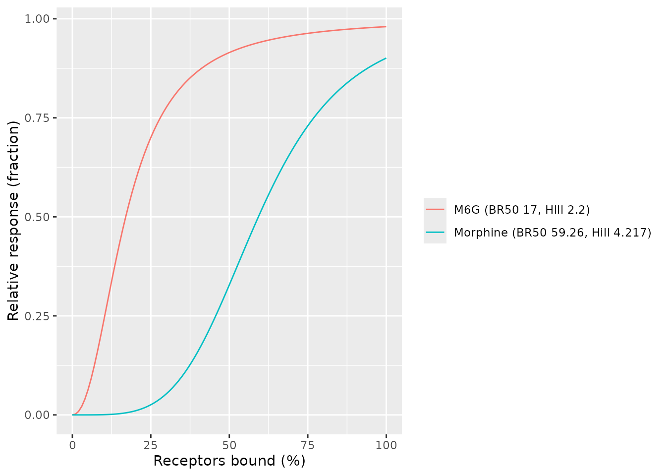

The time course of the morphine and M6G contributions after a 28 mg dose in a typical adult replicates the split shown in Figure 3B: the parent compound carries most of the response in the first hours.

ev_28 <- make_events(typ_adult, 28, iv_dur, obs_24)
s28 <- rxode2::rxSolve(mod_typ, ev_28, returnType = "data.frame")
#> ℹ omega/sigma items treated as zero: 'etalcl', 'etalcl_m6g', 'etalq_csf_prod', 'etalf_bulk', 'etalf_ssink', 'etalf_sout', 'etalhct'
s28 |>
  select(time, Morphine = rr, M6G = rr_m6g) |>
  pivot_longer(-time, names_to = "analyte", values_to = "response") |>
  ggplot(aes(time, response, colour = analyte)) +
  geom_line() +
  labs(x = "Time (h)", y = "Relative response (fraction)", colour = NULL)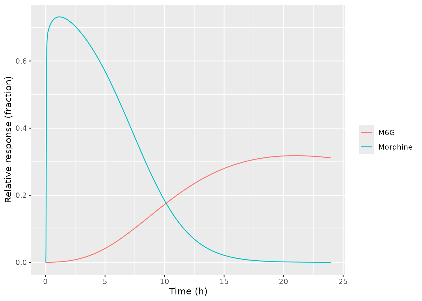


stopifnot(max(s28$rr) > max(s28$rr_m6g))

Assumptions and deviations

Adult physiology. The deposited code is the paediatric (2.6-16.4 y) version. Adult organ volumes, flows, haematocrit and tissue composition come from the adult column of the 2019 framework S1 Table, which the paper names as the source for its adult version.
Age boundaries. Adult equations apply from 18 y. Neonatal clearance, M6G formation fraction and the 10 mL/h CSF production apply below 0.25 y; the paper does not state its neonatal cut-off.
Pgp maturation shape. The paper gives two anchors (41% of adult at term, 100% at 6 months). Linear interpolation between them is assumed.
Adult virtual demographics. The deposited code has no adult height or weight generator. Adults here have height N(178, 7) cm (men) or N(165, 7) cm (women) and log-normal weight with medians of 80 kg and 66 kg and a 15% CV. The paper’s sex ratios were not reported in the article, so every arm is 50% female.
Dose administration. “Single IV dose” is simulated as a 5-min infusion into venous blood. This keeps the early peaks seen at the start of the Figure 2A and 2B profiles, and avoids the artificial venous spike a true bolus puts into the 2-3 L venous compartment at time zero. The deposited example code uses a 1-h infusion (tend = 1) for its own scenario. The paediatric ECF scenario (0.03 mg/kg/h) is simulated as a 24-h infusion for the cohort and a 100-h infusion for the typical-child check; the infusion length in the source study is not given in the article.
Clearance placement. The 2021 S1 File subtracts the cleared morphine (CL x venous concentration) from the arterial compartment. The model here removes it from venous blood, as in the 2019 framework code. The section “Clearance placement” above shows that the deposited form falls below the paper’s own Figures 2A and 2D, while the venous form reproduces them. The same placement is used for M6G.
CSF sampling site. Ventricular-drain samples (adults) are compared with the cranial CSF compartment, and lumbar-puncture samples (children) with the spinal CSF compartment.
Cohort size. The paper simulated 500 individuals per scenario; this vignette uses 100 per arm.
Observed data. The observed verification points of Figures 1-2 were not digitised. The simulated typical-value curves of Figure 2D and the median plateaus of the Figure 2A 9.5-year-old panels were digitised by the maintainers from the published figure, to check the clearance placement.
IIV. The model’s random effects reproduce the variability of the deposited virtual-population code (log-normal SDs as variances). The female haematocrit SD (0.071) is reached by rescaling the shared haematocrit eta.
Residual error. None was reported. propSd is fixed to 0 so the model can be used for estimation-style workflows.
Pharmacodynamics. The model returns the relative response (effect_rel, the sum of the morphine and M6G terms). The paper multiplies it by the maximum effect observed in each clinical study; that study-specific scaling is not part of the model.