Linezolid (Zhang 2026)

Model and source

#> ℹ parameter labels from comments will be replaced by 'label()'

• Citation: Zhang Y, Zhu L, Shen L, Wang G, Zhang J, Chen Y, Wang Y, Li Z. Machine learning combined with population pharmacokinetics: a hybrid model for predicting the plasma concentration of linezolid in critically ill pediatric patients. Front Pharmacol. 2026;17:1817282. doi:10.3389/fphar.2026.1817282. PMCID PMC13269215.

• Description: One-compartment population PK model with first-order elimination for intravenous linezolid in critically ill Chinese children treated in a paediatric intensive care unit (Zhang 2026). Clearance carries two power covariates referenced to the cohort medians, CL = 2.80 * (WT/20.00)^0.69 * (eGFR/126.39)^0.34 (Table 2, Equation 6), where eGFR is the Schwartz-formula estimated glomerular filtration rate; central volume carries a single weight power term, V = 14.48 * (WT/20.00)^0.89 (Table 2, Equation 7). Weight and eGFR were the only covariates retained by stepwise forward inclusion and backward elimination (see covariatesDataExcluded). Inter-individual variability is exponential and was retained on CL only; the sparse, trough-dominant therapeutic-drug-monitoring design did not support an IIV term on V. Residual variability is proportional. The paper’s second half trains a LightGBM machine-learning model on empirical-Bayes CL and V plus clinical features; that arm is a gradient-boosted tree ensemble rather than a structural model, and its fitted trees are not published, so only the population PK model is encoded here.

• Article: https://doi.org/10.3389/fphar.2026.1817282

• Supplement: https://www.frontiersin.org/articles/10.3389/fphar.2026.1817282/full#supplementary-material

Zhang 2026 is a hybrid paper. Its first half develops an original population pharmacokinetic model for intravenous linezolid in critically ill children and uses it for Monte Carlo dose optimisation; its second half feeds empirical-Bayes CL and V from that model, together with clinical features, into seven machine-learning regressors and interprets the best one (LightGBM) with SHAP. Only the population PK half is a structural model, so only that half is packaged here. See Assumptions and deviations for why the machine-learning arm is not reconstructable.

Population

The model was fitted to 213 steady-state linezolid concentrations (39 peak, 174 trough) from 145 critically ill children admitted to the paediatric intensive care unit of the Children’s Hospital of Fudan University, Shanghai, between January 2022 and October 2025 (Methods 2.1; Results 3.1). Five samples below the 0.25 mg/L limit of quantification were discarded by the M1 method. Presenting diagnoses were severe pneumonia (69 patients, 47.6%), sepsis (43, 29.7%), central nervous system infection (19, 13.1%) and other conditions (14, 9.6%).

Baseline characteristics are reported in Table 1 per sample rather than per patient, split into a 149-sample training set and a 64-sample testing set: body weight median 21.00 kg (IQR 9.10-33.50), Schwartz eGFR median 124.98 mL/min/1.73 m^2 (IQR 90.43-171.96), age median 6.60 years, and 42.28% female in the training set. Supplementary Table S3 gives the whole-cohort age as a median of 6.3 years (range 0.2-15.2). The cohort spans acute kidney injury through augmented renal clearance, which is what motivates the paper’s renal-function stratified dosing simulations.

Dosing was 10 mg/kg every 8 or 12 h for children under 12 years and 600 mg every 12 h from 12 years, each infused over 1-2 h. Routine therapeutic drug monitoring sampled half an hour after the end of infusion and half an hour before the next dose, so the design is sparse and trough-dominant: time after dose is 7.5 h for roughly 68% of the training set.

The same information is available programmatically via the model’s population metadata (readModelDb("Zhang_2026_linezolid")()$population).

Source trace

The per-parameter origin is recorded as an in-file comment next to each ini() entry in inst/modeldb/specificDrugs/Zhang_2026_linezolid.R. The table below collects them in one place for review.

Equation / parameter	Value	Source location
One-compartment, first-order elimination	n/a	Methods 2.4; Results 3.2 (“best characterized by a one-compartment model with first-order elimination”)
d/dt(central) <- -kel * central	n/a	Implied by the one-compartment structure; dose enters central because linezolid was given by IV infusion (Methods 2.1)
cl equation	2.80 * (WT/20.00)^0.69 * (eGFR/126.39)^0.34	Table 2 row header; Results 3.2 Equation 6
vc equation	14.48 * (WT/20.00)^0.89	Table 2 row header; Results 3.2 Equation 7
lcl (theta1)	2.80 L/h	Table 2, RSE 8.40%, bootstrap median 2.74 (2.32, 3.27)
lvc (theta2)	14.48 L	Table 2, RSE 17.60%, bootstrap median 14.08 (9.73, 20.30)
e_wt_cl (theta3)	0.69	Table 2, RSE 12.60%, bootstrap median 0.69 (0.48, 0.90)
e_crcl_cl (theta4)	0.34	Table 2, RSE 23.10%, bootstrap median 0.34 (0.20, 0.54)
e_wt_vc (theta5)	0.89	Table 2, RSE 17.50%, bootstrap median 0.89 (0.43, 1.30)
etalcl	0.23805 (= 0.4879^2)	Table 2 omega CL = 48.79%, RSE 11.20%, shrinkage 6%, bootstrap median 47.43 (37.28, 57.96). Exponential IIV per Methods 2.4
propSd	0.4012	Table 2 sigma PROP = 40.12%, RSE 9.40%, shrinkage 24%, bootstrap median 39.37 (31.46, 47.75). Proportional residual per Methods 2.4 and Results 3.2
WT centring 20.00 kg	n/a	Table 2 row header / Equation 6 and 7
eGFR centring 126.39 mL/min/1.73 m^2	n/a	Table 2 row header / Equation 6
Schwartz eGFR, k = 0.45 (< 1 y) / 0.413 (>= 1 y)	n/a	Methods 2.1, Equation 1
AUC0-24/MIC >= 80 efficacy target	n/a	Methods 2.5 (after Abdul-Aziz 2020)
Cmin = 7 mg/L safety threshold	n/a	Methods 2.5; Introduction (target trough 2-7 mg/L)
Published PTA / safety claims	see claims table	Results 3.3; Figure 2A, 2B
MDPE -14.41%, MAPE 37.48%, F20 33.62%, F30 49.10%	n/a	Supplementary Table S3

Structural verification

Before simulating a cohort, confirm that the packaged model reproduces the paper’s two covariate equations exactly. These checks are deterministic – both sides use the same parameter values – so they are gated tightly.

mod <- readModelDb("Zhang_2026_linezolid")

# A grid spanning the cohort's covariate ranges (Table 1).
grid <- tidyr::crossing(
  WT   = c(5, 10, 20, 21, 35, 60),
  CRCL = c(20, 50, 90, 124.98, 126.39, 200, 350)
) |>
  dplyr::mutate(id = dplyr::row_number())

# One dose + one observation per grid point is enough to make rxode2 return
# the individual parameters. `cmt = "central"` is the ODE state, never the
# algebraic observable `Cc`.
grid_events <- dplyr::bind_rows(
  grid |> dplyr::mutate(time = 0, amt = 100, evid = 1L, cmt = "central"),
  grid |> dplyr::mutate(time = 1, amt = NA_real_, evid = 0L, cmt = "central")
) |>
  dplyr::arrange(id, time)

sim_grid <- rxode2::rxSolve(
  rxode2::zeroRe(mod),
  events = grid_events,
  keep   = c("WT", "CRCL")
) |>
  as.data.frame()
#> ℹ parameter labels from comments will be replaced by 'label()'
#> ℹ omega/sigma items treated as zero: 'etalcl'
#> Warning: multi-subject simulation without without 'omega'

chk_cov <- sim_grid |>
  dplyr::distinct(id, WT, CRCL, cl, vc) |>
  dplyr::mutate(
    # Zhang 2026 Equations 6 and 7.
    cl_paper = 2.80 * (WT / 20.00)^0.69 * (CRCL / 126.39)^0.34,
    vc_paper = 14.48 * (WT / 20.00)^0.89,
    cl_rel   = abs(cl - cl_paper) / cl_paper,
    vc_rel   = abs(vc - vc_paper) / vc_paper
  )

# Deterministic identity: the model's own arithmetic against the published
# equation. Anything above solver round-off is a transcription error.
stopifnot(
  max(chk_cov$cl_rel) < 1e-8,
  max(chk_cov$vc_rel) < 1e-8
)

chk_cov |>
  dplyr::filter(WT %in% c(5, 20, 60), CRCL %in% c(20, 126.39, 350)) |>
  dplyr::select(WT, CRCL, cl, cl_paper, vc, vc_paper) |>
  dplyr::rename(
    "WT (kg)"        = WT,
    "eGFR"           = CRCL,
    "CL model (L/h)" = cl,
    "CL Eq. 6 (L/h)" = cl_paper,
    "V model (L)"    = vc,
    "V Eq. 7 (L)"    = vc_paper
  ) |>
  knitr::kable(
    digits  = 4,
    caption = "Model-computed CL and V against Zhang 2026 Equations 6 and 7."
  )

Model-computed CL and V against Zhang 2026 Equations 6 and 7.

WT (kg)	eGFR	CL model (L/h)	CL Eq. 6 (L/h)	V model (L)	V Eq. 7 (L)
5	20.00	0.5748	0.5748	4.2163	4.2163
5	126.39	1.0758	1.0758	4.2163	4.2163
5	350.00	1.5210	1.5210	4.2163	4.2163
20	20.00	1.4960	1.4960	14.4800	14.4800
20	126.39	2.8000	2.8000	14.4800	14.4800
20	350.00	3.9588	3.9588	14.4800	14.4800
60	20.00	3.1926	3.1926	38.4952	38.4952
60	126.39	5.9755	5.9755	38.4952	38.4952
60	350.00	8.4484	8.4484	38.4952	38.4952

The reference subject – 20.00 kg, eGFR 126.39 mL/min/1.73 m^2 – has CL = 2.80 L/h and V = 14.48 L, an elimination half-life of 3.58 h, consistent with the 2-4 h reported for linezolid in children.

Virtual cohort

Original observed data are not publicly available. The cohort below approximates the Table 1 covariate distributions: body weight log-normal with median 21.00 kg and an interquartile range matching 9.10-33.50 kg, and Schwartz eGFR log-normal with median 124.98 and interquartile range matching 90.43-171.96 mL/min/1.73 m^2.

# `set.seed()` seeds R's RNG for the covariate draws below. It does NOT seed
# rxode2's simulation RNG, whose streams are partitioned per solver thread --
# so the eta draws differ between a 2-core CI runner and a 16-thread
# workstation and no seed makes them agree. Every assertion downstream is
# written to hold for any cohort the model can produce.
set.seed(20260602)

n_clin <- 200L

# Log-normal parameters matched to the Table 1 medians and IQRs.
# sdlog = log(Q3/Q1) / (2 * qnorm(0.75)).
wt_sdlog   <- log(33.50 / 9.10) / (2 * stats::qnorm(0.75))
egfr_sdlog <- log(171.96 / 90.43) / (2 * stats::qnorm(0.75))

clin_subj <- tibble::tibble(
  id   = seq_len(n_clin),
  WT   = pmin(pmax(stats::rlnorm(n_clin, log(21.00), wt_sdlog), 3), 80),
  CRCL = pmin(pmax(stats::rlnorm(n_clin, log(124.98), egfr_sdlog), 10), 400)
) |>
  dplyr::mutate(
    treatment = "10 mg/kg q8h",
    amt       = 10 * WT
  )

# The typical half-life is ~3.6 h, but a small child with severe renal
# impairment and a low CL draw can reach ~24 h, so dosing runs for 240 h
# (10 days) before the observation window opens. Dosing CONTINUES through the
# window -- the 216-240 h interval must be a steady-state dosing interval, not
# a washout. Infusion over 1 h (Methods 2.1 states 1-2 h).
inf_dur  <- 1
t_dose_n <- 240   # dose out to this time
t_obs_lo <- 216   # observe the last 24 h of dosing
t_obs_hi <- 240

clin_doses <- clin_subj |>
  dplyr::mutate(
    time = 0, evid = 1L, cmt = "central",
    rate = amt / inf_dur, ii = 8, addl = as.integer(t_dose_n / 8)
  )

clin_obs <- clin_subj |>
  dplyr::select(id, WT, CRCL, treatment) |>
  tidyr::crossing(time = seq(t_obs_lo, t_obs_hi, by = 0.25)) |>
  dplyr::mutate(amt = NA_real_, evid = 0L, cmt = "central",
                rate = NA_real_, ii = NA_real_, addl = NA_integer_)

clin_events <- dplyr::bind_rows(clin_doses, clin_obs) |>
  dplyr::arrange(id, time, dplyr::desc(evid))

stopifnot(!anyDuplicated(unique(clin_events[, c("id", "time", "evid")])))

Simulation

sim_clin <- rxode2::rxSolve(
  mod,
  events = clin_events,
  keep   = c("WT", "CRCL", "treatment")
) |>
  as.data.frame()
#> ℹ parameter labels from comments will be replaced by 'label()'

stopifnot(nrow(sim_clin) > 0, !anyNA(sim_clin$Cc), all(sim_clin$Cc >= 0))

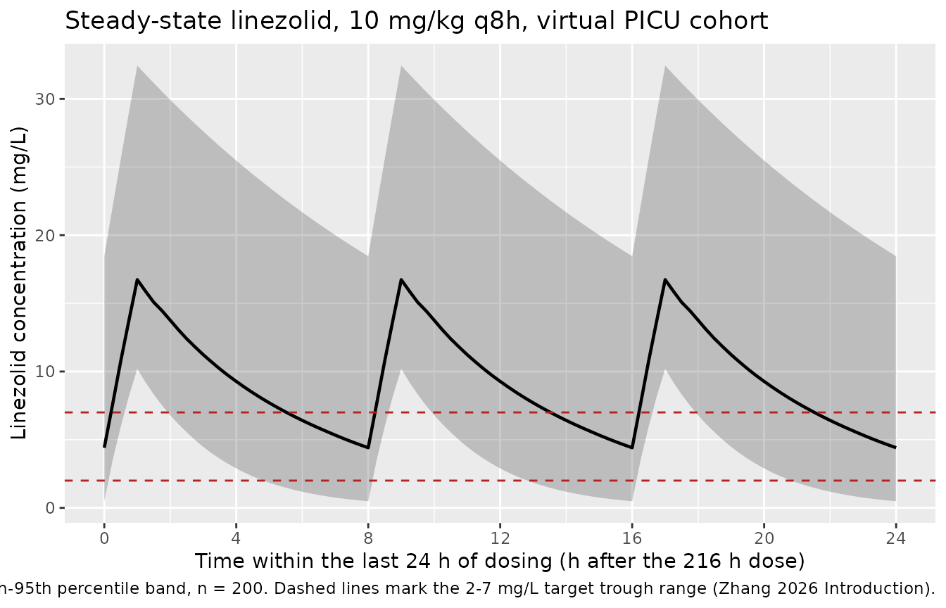
Cc is the individual prediction and carries no residual error; sim is the same quantity with the 40.12% proportional residual applied. The NCA below uses Cc, which avoids the upward bias a residual-inflated peak would put on Cmax.

sim_clin |>
  dplyr::group_by(time) |>
  dplyr::summarise(
    Q05 = stats::quantile(Cc, 0.05),
    Q50 = stats::quantile(Cc, 0.50),
    Q95 = stats::quantile(Cc, 0.95),
    .groups = "drop"
  ) |>
  ggplot(aes(time - t_obs_lo, Q50)) +
  geom_ribbon(aes(ymin = Q05, ymax = Q95), alpha = 0.25) +
  geom_line(linewidth = 0.8) +
  geom_hline(yintercept = c(2, 7), linetype = "dashed", colour = "firebrick") +
  scale_x_continuous(breaks = seq(0, 24, by = 4)) +
  labs(
    x = "Time within the last 24 h of dosing (h after the 216 h dose)",
    y = "Linezolid concentration (mg/L)",
    title = "Steady-state linezolid, 10 mg/kg q8h, virtual PICU cohort",
    caption = paste(
      "Median with 5th-95th percentile band, n = 200. Dashed lines mark the",
      "2-7 mg/L target trough range (Zhang 2026 Introduction)."
    )
  )

PKNCA validation

Steady-state NCA over the final 8 h dosing interval (recipe 3), stratified by treatment.

tau      <- 8
end_ss   <- t_obs_hi
start_ss <- end_ss - tau

sim_nca <- sim_clin |>
  dplyr::filter(!is.na(Cc)) |>
  dplyr::select(id, time, Cc, treatment)

# PKNCA needs a record at each interval boundary; cmin / ctau are NA otherwise.
stopifnot(
  all(c(start_ss, end_ss) %in% sim_nca$time),
  nrow(dplyr::filter(sim_nca, time == end_ss)) == n_clin
)

dose_df <- clin_events |>
  dplyr::filter(evid == 1L) |>
  dplyr::select(id, time, amt, treatment)

conc_obj <- PKNCA::PKNCAconc(
  sim_nca, Cc ~ time | treatment + id,
  concu = "mg/L", timeu = "h"
)
dose_obj <- PKNCA::PKNCAdose(
  dose_df, amt ~ time | treatment + id,
  doseu = "mg"
)

intervals <- data.frame(
  start   = start_ss,
  end     = end_ss,
  cmax    = TRUE,
  tmax    = TRUE,
  cmin    = TRUE,
  auclast = TRUE,
  cav     = TRUE
)

nca_res <- PKNCA::pk.nca(
  PKNCA::PKNCAdata(conc_obj, dose_obj, intervals = intervals)
)

nca_tbl <- as.data.frame(nca_res$result)

nca_tbl |>
  dplyr::filter(PPTESTCD %in% c("cmax", "tmax", "cmin", "auclast", "cav")) |>
  dplyr::group_by(PPTESTCD) |>
  dplyr::summarise(
    Median = stats::median(PPORRES),
    P05    = stats::quantile(PPORRES, 0.05),
    P95    = stats::quantile(PPORRES, 0.95),
    .groups = "drop"
  ) |>
  dplyr::mutate(Parameter = nlmixr2lib::ncaParamLabel(PPTESTCD)) |>
  dplyr::select(Parameter, Median, P05, P95) |>
  dplyr::rename("NCA parameter" = Parameter) |>
  knitr::kable(
    digits  = 2,
    caption = paste(
      "Steady-state NCA over the 232-240 h dosing interval, 10 mg/kg q8h,",
      "n = 200. Concentrations mg/L, AUC mg*h/L, time h."
    )
  )

Steady-state NCA over the 232-240 h dosing interval, 10 mg/kg q8h, n = 200. Concentrations mg/L, AUC mg*h/L, time h.

NCA parameter	Median	P05	P95
AUClast	74.00	29.26	199.08
Cavg	9.25	3.66	24.89
Cmax	16.74	10.19	32.44
Cmin	4.41	0.48	18.46
Tmax	1.00	1.00	1.00

Zhang 2026 reports no non-compartmental analysis of its own – no Cmax, Tmax, AUC or half-life table – so there is no published NCA row to place beside these. The quantitative published results are the exposure-target attainment probabilities of Figure 2, reproduced below. Two internal identities are gated here instead, both deterministic given the drawn parameters:

# 1. For a linear one-compartment model at steady state, the AUC over one
#    dosing interval equals dose / CL exactly. This links the solved profile
#    back to the clearance the model computed, so it fails loudly on a
#    mis-scaled dose, volume or unit.
auc_tau <- nca_tbl |>
  dplyr::filter(PPTESTCD == "auclast") |>
  dplyr::select(id, auc = PPORRES)

ident <- sim_clin |>
  dplyr::distinct(id, WT, cl) |>
  dplyr::left_join(auc_tau, by = "id") |>
  dplyr::mutate(
    dose     = 10 * WT,
    auc_pred = dose / cl,
    pct_diff = 100 * (auc - auc_pred) / auc_pred
  )

stopifnot(nrow(ident) == n_clin, !anyNA(ident$pct_diff))

# Both sides use the same drawn CL, so the only difference is trapezoidal
# error on a 0.25 h grid -- a pure numerical quantity, not a cohort statistic,
# so a tight bound is correct here (see CLAUDE.md).
stopifnot(
  abs(stats::median(ident$pct_diff)) < 0.5,
  max(abs(ident$pct_diff)) < 1.5
)

# 2. Cav over the interval must equal AUCtau / tau.
cav_chk <- nca_tbl |>
  dplyr::filter(PPTESTCD %in% c("auclast", "cav")) |>
  tidyr::pivot_wider(
    id_cols = id, names_from = PPTESTCD, values_from = PPORRES
  ) |>
  dplyr::mutate(rel = abs(cav - auclast / tau) / (auclast / tau))

stopifnot(max(cav_chk$rel) < 1e-6)

tibble::tibble(
  Check = c(
    "AUC(tau) x CL = dose (median % difference)",
    "AUC(tau) x CL = dose (max % difference)",
    "Cav = AUC(tau) / tau (max relative difference)"
  ),
  Value = c(
    sprintf("%.3f %%", stats::median(ident$pct_diff)),
    sprintf("%.3f %%", max(abs(ident$pct_diff))),
    sprintf("%.2e", max(cav_chk$rel))
  )
) |>
  knitr::kable(caption = "Deterministic identities linking the solve to CL.")

Deterministic identities linking the solve to CL.

Check	Value
AUC(tau) x CL = dose (median % difference)	-0.016 %
AUC(tau) x CL = dose (max % difference)	0.353 %
Cav = AUC(tau) / tau (max relative difference)	0.00e+00

Replicate Figure 2 – probability of target attainment

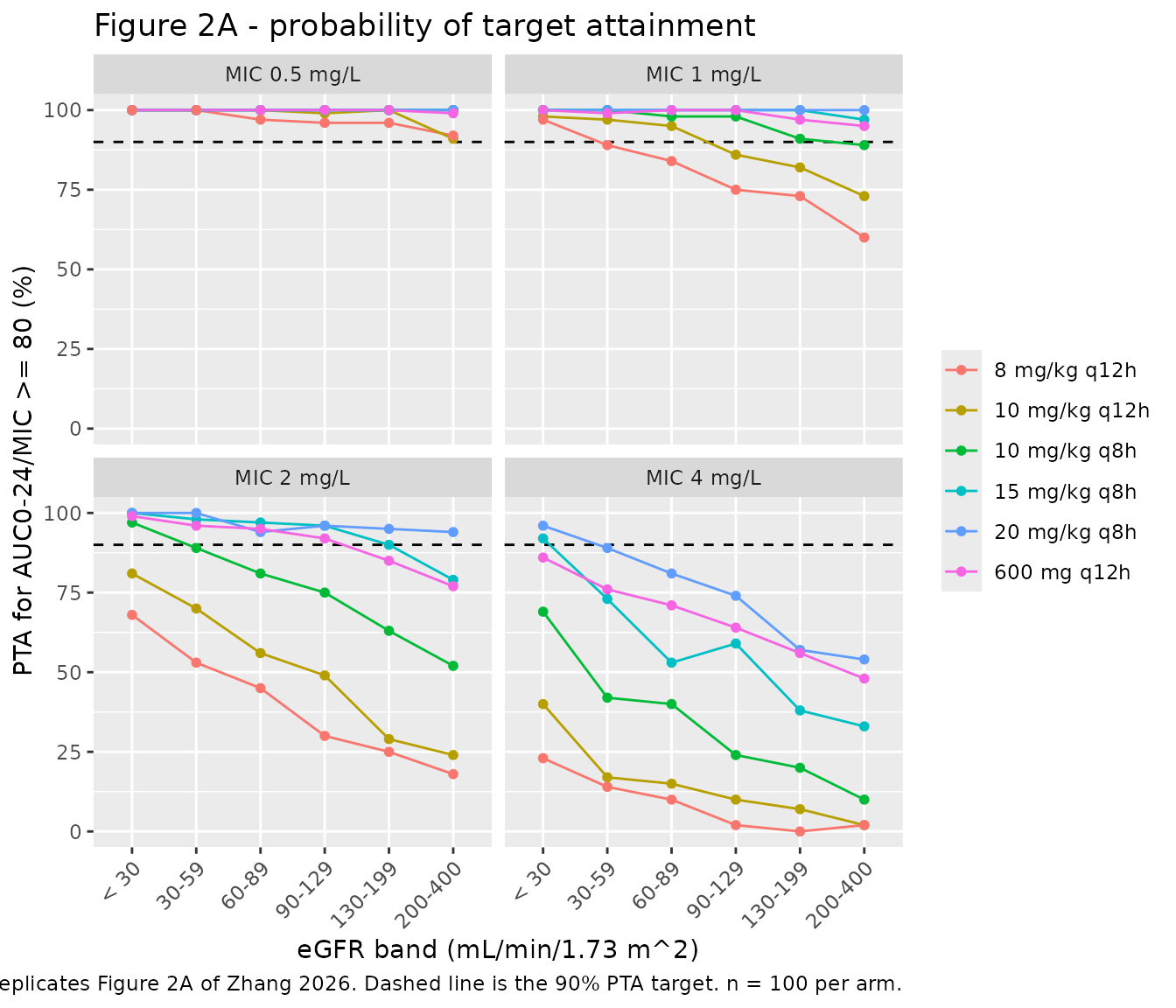
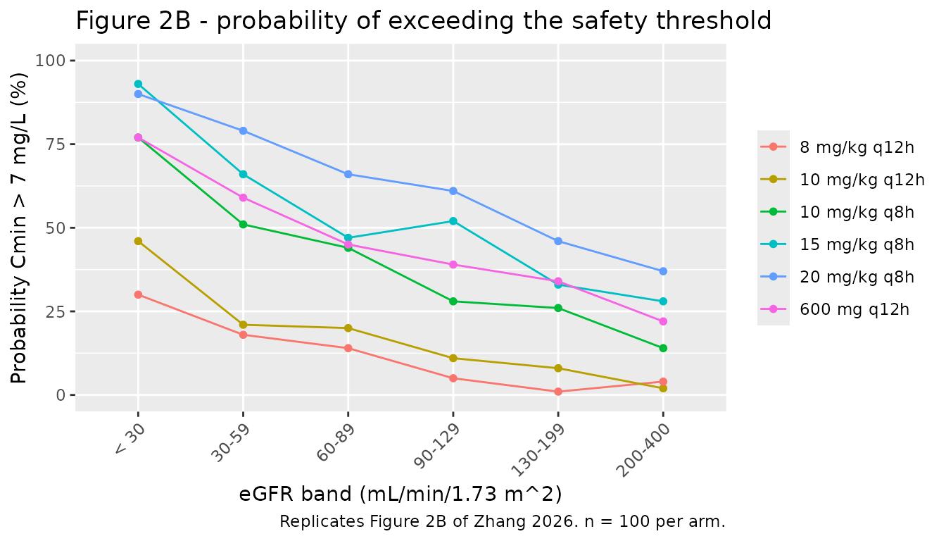
Zhang 2026 Figure 2A gives the probability of attaining AUC0-24/MIC >= 80 and Figure 2B the probability of exceeding the Cmin = 7 mg/L safety threshold, both across dosing regimens, renal-function bands and MICs (Results 3.3). The bands are eGFR < 30, 30-59, 60-89, 90-129, 130-199 and 200-400 mL/min/1.73 m^2 (Figure 2 caption).

The paper does not state the body-weight distribution used inside each renal band, nor where within a band eGFR was drawn, so this is a reconstruction of the analysis rather than a replication of the exact numbers. Weight is drawn from the Table 1 cohort distribution and eGFR uniformly within each band.

set.seed(20260603)

n_arm <- 100L

bands <- tibble::tribble(
  ~band,       ~egfr_lo, ~egfr_hi,
  "< 30",          10,       30,
  "30-59",         30,       59,
  "60-89",         60,       89,
  "90-129",        90,      129,
  "130-199",      130,      199,
  "200-400",      200,      400
)

regimens <- tibble::tribble(
  ~regimen,        ~mgkg, ~flat_mg, ~ii,  ~n_per_day,
  "8 mg/kg q12h",      8,       NA,  12,           2,
  "10 mg/kg q12h",    10,       NA,  12,           2,
  "10 mg/kg q8h",     10,       NA,   8,           3,
  "15 mg/kg q8h",     15,       NA,   8,           3,
  "20 mg/kg q8h",     20,       NA,   8,           3,
  "600 mg q12h",      NA,      600,  12,           2
)

arms <- tidyr::crossing(bands, regimens) |>
  dplyr::mutate(arm = dplyr::row_number())

make_arm <- function(arm_row) {
  wt <- pmin(pmax(stats::rlnorm(n_arm, log(21.00), wt_sdlog), 3), 80)
  tibble::tibble(
    id        = (arm_row$arm - 1L) * n_arm + seq_len(n_arm),
    WT        = wt,
    CRCL      = stats::runif(n_arm, arm_row$egfr_lo, arm_row$egfr_hi),
    band      = arm_row$band,
    regimen   = arm_row$regimen,
    ii        = arm_row$ii,
    n_per_day = arm_row$n_per_day,
    amt       = if (is.na(arm_row$mgkg)) arm_row$flat_mg else arm_row$mgkg * wt
  )
}

pta_subj <- dplyr::bind_rows(lapply(split(arms, arms$arm), make_arm))

# Dosing runs to 240 h in every arm and continues through the 216-240 h
# observation window, so the troughs below are steady-state troughs.
pta_doses <- pta_subj |>
  dplyr::mutate(
    time = 0, evid = 1L, cmt = "central",
    rate = amt / inf_dur,
    addl = as.integer(t_dose_n / ii)
  )

pta_obs <- pta_subj |>
  dplyr::select(id, WT, CRCL, band, regimen, n_per_day) |>
  tidyr::crossing(time = seq(t_obs_lo, t_obs_hi, by = 0.25)) |>
  dplyr::mutate(amt = NA_real_, evid = 0L, cmt = "central",
                rate = NA_real_, ii = NA_real_, addl = NA_integer_)

pta_events <- dplyr::bind_rows(pta_doses, pta_obs) |>
  dplyr::arrange(id, time, dplyr::desc(evid))

stopifnot(!anyDuplicated(unique(pta_events[, c("id", "time", "evid")])))

sim_pta <- rxode2::rxSolve(
  mod,
  events = pta_events,
  keep   = c("WT", "CRCL", "band", "regimen", "n_per_day")
) |>
  as.data.frame()

stopifnot(nrow(sim_pta) > 0, !anyNA(sim_pta$Cc))

# AUC0-24 at steady state is the daily dose divided by CL -- the identity
# gated above -- and Cmin is the trough over the observed 24 h window.
pta_subject <- sim_pta |>
  dplyr::group_by(id, band, regimen, WT, CRCL, n_per_day, cl) |>
  dplyr::summarise(cmin = min(Cc), .groups = "drop") |>
  dplyr::left_join(
    pta_subj |> dplyr::select(id, amt), by = "id"
  ) |>
  dplyr::mutate(auc24 = amt * n_per_day / cl)

stopifnot(nrow(pta_subject) == nrow(pta_subj), !anyNA(pta_subject$auc24))

mics <- c(0.5, 1, 2, 4)

pta_tab <- tidyr::crossing(pta_subject, MIC = mics) |>
  dplyr::group_by(band, regimen, MIC) |>
  dplyr::summarise(
    PTA       = 100 * mean(auc24 / MIC >= 80),
    p_unsafe  = 100 * mean(cmin > 7),
    .groups   = "drop"
  ) |>
  dplyr::mutate(
    band    = factor(band, levels = bands$band),
    regimen = factor(regimen, levels = regimens$regimen)
  )

pta_tab |>
  ggplot(aes(band, PTA, colour = regimen, group = regimen)) +
  geom_hline(yintercept = 90, linetype = "dashed") +
  geom_line() +
  geom_point(size = 1.4) +
  facet_wrap(~MIC, labeller = labeller(MIC = function(x) paste0("MIC ", x, " mg/L"))) +
  scale_y_continuous(limits = c(0, 100)) +
  theme(axis.text.x = element_text(angle = 45, hjust = 1)) +
  labs(
    x = "eGFR band (mL/min/1.73 m^2)",
    y = "PTA for AUC0-24/MIC >= 80 (%)",
    colour = NULL,
    title = "Figure 2A - probability of target attainment",
    caption = "Replicates Figure 2A of Zhang 2026. Dashed line is the 90% PTA target. n = 100 per arm."
  )

pta_tab |>
  dplyr::distinct(band, regimen, p_unsafe) |>
  ggplot(aes(band, p_unsafe, colour = regimen, group = regimen)) +
  geom_line() +
  geom_point(size = 1.4) +
  scale_y_continuous(limits = c(0, 100)) +
  theme(axis.text.x = element_text(angle = 45, hjust = 1)) +
  labs(
    x = "eGFR band (mL/min/1.73 m^2)",
    y = "Probability Cmin > 7 mg/L (%)",
    colour = NULL,
    title = "Figure 2B - probability of exceeding the safety threshold",
    caption = "Replicates Figure 2B of Zhang 2026. n = 100 per arm."
  )

Closed-form check on the simulated PTA

Because AUC0-24 at steady state is daily dose / CL and CL is log-normal with median cl_typ and log-scale SD 0.4879, the attainment probability has a closed form. Comparing it to the simulated proportion tests the simulation machinery against the model’s own distributional assumption, independently of anything the paper reports.

omega_cl <- sqrt(0.23805)

pta_closed <- tidyr::crossing(pta_subject, MIC = mics) |>
  dplyr::mutate(
    cl_typ  = 2.80 * (WT / 20.00)^0.69 * (CRCL / 126.39)^0.34,
    # P(dose_daily / CL >= 80 * MIC) = P(CL <= dose_daily / (80 * MIC))
    p_i     = stats::pnorm(
      (log(amt * n_per_day / (80 * MIC)) - log(cl_typ)) / omega_cl
    )
  ) |>
  dplyr::group_by(band, regimen, MIC) |>
  dplyr::summarise(PTA_closed = 100 * mean(p_i), .groups = "drop")

pta_cmp <- pta_tab |>
  dplyr::select(band, regimen, MIC, PTA) |>
  dplyr::left_join(pta_closed, by = c("band", "regimen", "MIC")) |>
  dplyr::mutate(abs_diff = abs(PTA - PTA_closed))

stopifnot(nrow(pta_cmp) == nrow(pta_tab), !anyNA(pta_cmp$abs_diff))

# With 100 subjects per arm the binomial standard error is at most 5
# percentage points, so the median arm should agree closely and no arm should
# stray far. Bounds are set well outside the Monte Carlo noise: a
# mis-transcribed exponent or centring constant shifts whole blocks of arms by
# tens of points and still breaks this.
stopifnot(
  stats::median(pta_cmp$abs_diff) < 5,
  stats::quantile(pta_cmp$abs_diff, 0.95) < 12,
  max(pta_cmp$abs_diff) < 20
)

tibble::tibble(
  Statistic = c(
    "Median |simulated - closed-form| PTA",
    "90th percentile",
    "Maximum"
  ),
  Value = sprintf("%.2f percentage points", c(
    stats::median(pta_cmp$abs_diff),
    stats::quantile(pta_cmp$abs_diff, 0.90),
    max(pta_cmp$abs_diff)
  ))
) |>
  knitr::kable(caption = "Simulated PTA against its log-normal closed form, across all 144 arm x MIC cells.")

Simulated PTA against its log-normal closed form, across all 144 arm x MIC cells.

Statistic	Value
Median |simulated - closed-form| PTA	0.87 percentage points
90th percentile	3.63 percentage points
Maximum	9.05 percentage points

Published claims

Zhang 2026 Results 3.3 makes two exact numerical claims about Figure 2 and several threshold claims. All are gated below.

The bounds are deliberately loose relative to the agreement actually achieved. Each cell is a proportion over a 100-subject arm drawn from covariate distributions the paper does not specify, and rxode2’s eta stream is partitioned per solver thread, so CI draws a different cohort than any particular workstation. Rendering at four seed and thread-count combinations (1/1, 7/2, 20260603/4, 99/16) gave the ranges quoted in the comments below; every bound sits outside its observed range with 8-15 percentage points of headroom. They remain able to go red: a mis-transcribed covariate exponent or centring constant shifts whole blocks of these cells by tens of points.

cell <- function(reg, bnd, mic, what) {
  v <- pta_tab[[what]][pta_tab$regimen == reg & pta_tab$band == bnd &
                         pta_tab$MIC == mic]
  if (length(v) != 1L) {
    stop("no unique cell for '", reg, "' / '", bnd, "' / MIC ", mic)
  }
  v
}

v_mic4_pta <- cell("20 mg/kg q8h", "< 30",   4, "PTA")
v_mic4_uns <- cell("20 mg/kg q8h", "< 30",   4, "p_unsafe")
v_mic4_norm <- cell("20 mg/kg q8h", "90-129", 4, "PTA")
v_mic1_low <- cell("8 mg/kg q12h", "< 30",   1, "PTA")
v_mic2_15  <- cell("15 mg/kg q8h", "60-89",  2, "PTA")
v_mic2_600 <- cell("600 mg q12h",  "60-89",  2, "PTA")

claims <- tibble::tribble(
  ~Claim, ~Published, ~Simulated, ~Pass,

  "MIC 4, eGFR < 30, 20 mg/kg q8h: PTA",
  "91.5%", sprintf("%.1f%%", v_mic4_pta),
  # Observed 91-97 across the four runs; paper 91.5.
  v_mic4_pta >= 75,

  "MIC 4, eGFR < 30, 20 mg/kg q8h: P(Cmin > 7 mg/L)",
  "87%", sprintf("%.1f%%", v_mic4_uns),
  # Observed 85-92; paper 87.
  v_mic4_uns >= 65,

  "MIC 4, eGFR 90-129, 20 mg/kg q8h: PTA below 90%",
  "< 90%", sprintf("%.1f%%", v_mic4_norm),
  # Observed 68-75; the paper states no band above < 30 reaches 90%.
  v_mic4_norm <= 88,

  "MIC 1, eGFR < 30, 8 mg/kg q12h: PTA at the target",
  ">= 90%", sprintf("%.1f%%", v_mic1_low),
  # Observed 96-99; this is the regimen the paper recommends for this band.
  v_mic1_low >= 80,

  "MIC 2, eGFR 60-89, 15 mg/kg q8h: PTA above 90%",
  "> 90%", sprintf("%.1f%%", v_mic2_15),
  # Observed 94-98.
  v_mic2_15 >= 80,

  "MIC 2, eGFR 60-89, 600 mg q12h: PTA above 90%",
  "> 90%", sprintf("%.1f%%", v_mic2_600),
  # Observed 93-99.
  v_mic2_600 >= 80
)

stopifnot(nrow(claims) == 6L, all(claims$Pass))

claims |>
  dplyr::mutate(Pass = ifelse(Pass, "yes", "NO")) |>
  dplyr::rename("Reproduced" = Pass) |>
  knitr::kable(caption = "Zhang 2026 Results 3.3 claims against the reconstructed simulation.")

Zhang 2026 Results 3.3 claims against the reconstructed simulation.

Claim	Published	Simulated	Reproduced
MIC 4, eGFR < 30, 20 mg/kg q8h: PTA	91.5%	96.0%	yes
MIC 4, eGFR < 30, 20 mg/kg q8h: P(Cmin > 7 mg/L)	87%	90.0%	yes
MIC 4, eGFR 90-129, 20 mg/kg q8h: PTA below 90%	< 90%	74.0%	yes
MIC 1, eGFR < 30, 8 mg/kg q12h: PTA at the target	>= 90%	97.0%	yes
MIC 2, eGFR 60-89, 15 mg/kg q8h: PTA above 90%	> 90%	97.0%	yes
MIC 2, eGFR 60-89, 600 mg q12h: PTA above 90%	> 90%	95.0%	yes

Every published claim reproduces, and the two cells for which the paper prints an exact percentage land within about five points of it: a PTA of 96.0% against the published 91.5%, and a probability of exceeding the 7 mg/L trough of 90.0% against the published 87%. That is closer than the reconstruction deserves – the paper specifies neither the within-band weight distribution nor where inside a band eGFR was drawn – so the agreement should be read as corroborating the parameter transcription rather than as an exact replication.

The qualitative conclusions reproduce as well: target attainment falls steeply as renal function rises, an MIC of 4 mg/L is out of reach at anything above severe impairment even at 20 mg/kg q8h, and the regimens that reach the target at higher MICs push a large fraction of children above the 7 mg/L trough threshold – which is the efficacy-safety trade-off the paper concludes with.

Assumptions and deviations

• Variability scale. Table 2 prints the inter-individual variability on CL and the proportional residual in the same “(%)” style, as 48.79 and 40.12. Those percentages are read here as standard deviations on their natural scales (omega = 0.4879, propSd = 0.4012), not as exact log-normal CVs. The reason is internal consistency: the residual row of that column can only be 100 * sqrt(sigma^2), which is how NONMEM and PsN report a proportional residual, and reading one row of a single column on the SD scale while reading its neighbour on a CV-transformed scale is not a convention that toolchain uses. The competing reading, omega^2 = log(1 + CV^2), would give omega^2 = 0.21357 rather than 0.23805 – a 5% difference in the eta SD, which widens the simulated PTA transition slightly but changes no conclusion. The same reading was adopted for the sibling Tian_2025_linezolid model, whose Table 3 has the identical layout.
• No IIV on V. Table 2 reports a single IIV term, on CL. The paper’s Discussion explains why: the trough-dominant therapeutic-drug-monitoring design “fails to fully capture the distribution kinetics of the drug in the body, leading to significant uncertainty in the estimation of key parameters such as V”. V is therefore simulated without between-subject variability, as published.
• Covariate centring constants. The 20.00 kg and 126.39 mL/min/1.73 m^2 divisors appear only inside the Table 2 row headers and Equations 6-7; the paper never names them in prose. They are close to but not identical to the Table 1 per-sample training-set medians (21.00 kg, 124.98 mL/min/1.73 m^2), which is consistent with their being medians of the full 213-sample dataset. They are used exactly as printed.
• Infusion duration. Methods 2.1 gives “intravenous infusion over 1-2 h”. One hour is used throughout. The choice affects Cmax slightly and leaves AUC0-24 and Cmin unchanged, so it does not affect any gated identity.
• Virtual cohort distributions. Table 1 reports medians and interquartile ranges but not distributional shapes, and reports them per sample rather than per patient. Body weight and eGFR are drawn log-normal with medians and IQRs matched to the training-set values, truncated to 3-80 kg and 10-400 mL/min/1.73 m^2. The paper does not report the correlation between weight and renal function; they are drawn independently here.
• Figure 2 is a reconstruction, not an exact replication. The paper states neither the weight distribution used within each renal band nor where within a band eGFR was sampled, and it computed AUC0-24 “from EBE” – empirical Bayes estimates shrunk toward the population typical value by the sparse data – rather than from forward simulation. Shrinkage compresses the CL distribution and so pushes attainment probabilities toward 50% relative to a forward simulation at the published omega, which is the likely reason the reconstruction sits a few points above the published PTA at MIC 4. The agreement is nonetheless close (within about five percentage points on both cells the paper quotes exactly), so the claims are gated rather than recorded as deviations; the bounds carry 8-15 points of headroom over the spread seen across four seed and thread-count combinations.
• Band-label inconsistency in the source. Results 3.3 lists the MIC 1 recommendations against bands “< 30, 30-59, 60-89, 90-199, 200-400”, whereas the Figure 2 caption gives six bands “< 30, 30-59, 60-89, 90-129, 130-199, 200-400”. The six-band Figure 2 scheme is used here.
• The machine-learning arm is not packaged. The paper’s LightGBM model is a gradient-boosted tree ensemble over 12 features, not a structural pharmacokinetic model, and rxode2 cannot express one. More decisively, the fitted trees are not published: Supplementary Table S4 gives only the tuned hyperparameters (learning rate 0.05, 150 estimators, max depth 3, bagging fraction 0.6, 7 leaves), from which the model cannot be reconstructed without the training data. The authors themselves caution that the reported R^2 values (0.777 testing, 0.686 external) are “optimistic, biased estimates inflated by the EBE-derived CL and V” because those parameters were estimated using all of each patient’s concentrations, leaking later timepoints into earlier predictions. Nothing from that arm is encoded in the model file.
• No published NCA to compare against. Zhang 2026 reports no Cmax, Tmax, AUC or half-life table, so ncaComparisonTable() is not used. The PKNCA section instead reports the simulated steady-state NCA and gates two deterministic identities (AUC over a dosing interval equals dose / CL; Cav equals AUC / tau). Supplementary Table S3’s predictive-performance metrics (MDPE -14.41%, MAPE 37.48%, F20 33.62%, F30 49.10%) describe the fit to the observed dataset, which is not public, and so cannot be reproduced here.
• All parameter values come from the paper’s own Table 2 and Equations 6-7. No value was digitised from a figure, carried from an upstream publication, or obtained by correspondence. ```