Ozanezumab (Berges 2015)
Source:vignettes/articles/Berges_2015_ozanezumab.Rmd
Berges_2015_ozanezumab.RmdModel and source
- Citation: Berges A, Bullman J, Bates S, Krull D, Williams N, Chen C. Ozanezumab Dose Selection for Amyotrophic Lateral Sclerosis by Pharmacokinetic-Pharmacodynamic Modelling of Immunohistochemistry Data from Patient Muscle Biopsies. PLoS ONE. 2015;10(2):e0117355. doi:10.1371/journal.pone.0117355
- Description: Two-compartment IV population PK plus effect-compartment sigmoid Emax PKPD model for the proportion of skeletal-muscle membrane Nogo-A co-localized with ozanezumab in adults with amyotrophic lateral sclerosis (ALS), based on the GlaxoSmithKline first-in-human study NCT00875446 (Berges 2015, Table 2)
- Article: https://doi.org/10.1371/journal.pone.0117355
Population
The model was developed from the first-in-human study NCT00875446 in adults with amyotrophic lateral sclerosis (ALS) (Berges 2015 Methods, Table 1). The study enrolled 76 subjects across eight cohorts. Part 1 was a single-dose ascending design with 5 cohorts each receiving 6 ozanezumab and 2 placebo subjects at single IV doses of 0.01, 0.1, 1.0, 5.0, or 15 mg/kg (infused over 1 hour). Part 2 was a repeat-dose design with 3 cohorts each receiving 9 ozanezumab and 3 placebo subjects at two IV doses of 0.5, 2.5, or 15 mg/kg given approximately 4 weeks apart. Plasma PK samples were collected in all dosed subjects at multiple post-dose time points (1, 10 and 24 h after dosing; 2, 4, 6, 8 and 12 weeks after dosing in Part 1; extended through week 16 in Part 2). The PD endpoint (percentage of skeletal-muscle membrane Nogo-A co-localized with ozanezumab, by IHC and laser scanning cytometry of deltoid biopsies) was obtained from pre-dose biopsies in cohorts 5-8 and post-dose biopsies in cohorts 7 and 8 only. Muscle samples from cohort 3 were unsuitable for IHC due to freeze artefacts and excluded from the PKPD analysis. Sex, age, race / ethnicity, weight range, and regional distribution are not tabulated in the paper.
The same information is available programmatically via
readModelDb("Berges_2015_ozanezumab")$population.
Source trace
Per-parameter origin is recorded as an in-file comment next to each
ini() entry in
inst/modeldb/specificDrugs/Berges_2015_ozanezumab.R. The
table below collects the origins for review. All structural and variance
parameters are from Berges 2015 Table 2; the equations are Berges 2015
Eqs. 1-4 in the “PKPD model” Results paragraph.
| Equation / parameter | Value | Source location |
|---|---|---|
| Structural model | 2-compartment IV PK + effect compartment + sigmoid Emax PD | Berges 2015 Results, “PKPD model”; Eqs. 1-4 |
lcl (CL) |
log(0.2808) L/day |
Table 2: CL = 11.7 mL/h (RSE 4.2%); converted to L/day |
lvc (Vc) |
log(3.31) L |
Table 2: Vc = 3310 mL (RSE 4.3%); converted to L |
lq (Q) |
log(0.3504) L/day |
Table 2: Q = 14.6 mL/h (RSE 8.6%); converted to L/day |
lvp (Vp) |
log(3.65) L |
Table 2: Vp = 3650 mL (RSE 5.0%); converted to L |
lke0 (ke0) |
log(0.08616) 1/day |
Table 2: ke0 = 0.00359 1/h (RSE 14%); converted to 1/day |
le0 (E0) |
log(6.04) % |
Table 2: E0 = 6.04 % (RSE 26%) |
lemax (Emax) |
fixed(log(100)) % |
Table 2: Emax = 100 % (Fixed) |
lec50 (EC50) |
log(24.9) ug/mL |
Table 2: EC50 = 24.9 ug/mL (RSE 10%) |
lgamma (Hill exponent) |
log(1.94) |
Table 2: gamma = 1.94 (RSE 14%) |
etalcl (BSV variance on CL) |
0.063 |
Table 2: variance 0.063 (CV 25%, RSE 21%) |
etalvc (BSV variance on Vc) |
0.0401 |
Table 2: variance 0.0401 (CV 20%, RSE 20%) |
propSd (PK proportional) |
0.254 |
Table 2: CV_PK = 25.4% (RSE 5.0%) |
addSd_nogoColoc (PD additive) |
6.16 % |
Table 2: Sigma PD = 38.0 (SD 6.16, RSE 56%) |
d/dt(central) |
2-cmt disposition with elimination from central | Eqs. 1-2 |
d/dt(effect) = ke0*(Cc - effect) |
effect-compartment delay | Eq. 3 |
nogoColoc = E0 + (Emax - E0) * Ce^gamma / (EC50^gamma + Ce^gamma) |
sigmoid Emax with E(0)=E0 and E(inf)=Emax | Eq. 4 (see Assumptions for the parameterisation choice) |
Virtual cohort
The published individual-level data are not available. The cohort below combines a typical 70 kg adult (for typical-value figures) with a virtual cohort of 200 subjects whose body weight follows a normal distribution truncated to a clinically plausible range. Body weight does not enter the structural model directly – ozanezumab CL, Vc, Q, Vp are absolute (mL/h and mL in the paper) – but it is required to translate the published mg/kg dose levels into absolute mg doses for the simulation.
set.seed(20150223) # paper publication date 2015-02-23

n_subj <- 200
adult_cohort <- tibble(
  id = seq_len(n_subj),
  WT = pmin(pmax(rnorm(n_subj, mean = 70, sd = 12), 45), 110)
)

typical_subject <- tibble(id = 1L, WT = 70)
Each subject in the simulations below receives an IV infusion of
ozanezumab over 1 hour into the central compartment, with
the absolute mg dose computed from the cohort’s body weight and the
published mg/kg level.
Simulation
mod <- rxode2::rxode2(readModelDb("Berges_2015_ozanezumab"))
#> ℹ parameter labels from comments will be replaced by 'label()'
mod_typical <- mod |> rxode2::zeroRe()

infusion_h    <- 1
infusion_day  <- infusion_h / 24

# Helper: build a dose + observation event table for one cohort at one mg/kg
# dose regimen (one or two doses, 4 weeks apart per Part 2 of the study). The
# observation grid is the same across cohorts so figures stack cleanly.
make_events <- function(cohort, dose_mg_per_kg, second_dose_day = NA_real_,
                        end_day = 84, obs_step = 0.5) {
  obs_times <- seq(0, end_day, by = obs_step)

  dose1 <- cohort |>
    dplyr::mutate(time = 0,
                  amt  = dose_mg_per_kg * WT,
                  rate = (dose_mg_per_kg * WT) / infusion_day,
                  cmt  = "central", evid = 1L)

  rows <- list(dose1)
  if (!is.na(second_dose_day)) {
    dose2 <- cohort |>
      dplyr::mutate(time = second_dose_day,
                    amt  = dose_mg_per_kg * WT,
                    rate = (dose_mg_per_kg * WT) / infusion_day,
                    cmt  = "central", evid = 1L)
    rows <- c(rows, list(dose2))
  }
  obs_cc <- cohort |>
    tidyr::crossing(time = obs_times) |>
    dplyr::mutate(amt = 0, rate = 0, cmt = "Cc", evid = 0L)
  obs_pd <- cohort |>
    tidyr::crossing(time = obs_times) |>
    dplyr::mutate(amt = 0, rate = 0, cmt = "nogoColoc", evid = 0L)
  rows <- c(rows, list(obs_cc, obs_pd))

  dplyr::bind_rows(rows) |>
    dplyr::select(id, time, amt, rate, cmt, evid, WT) |>
    dplyr::arrange(id, time, dplyr::desc(evid))
}

# Compartment ordering follows the d/dt() and observation-equation declaration
# order in model(): central=1, peripheral1=2, effect=3, Cc=4, nogoColoc=5.
cmt_cc        <- 4L
cmt_nogoColoc <- 5L
Replicate published figures
Figure 1, top panel: plasma PK after repeat dosing
Berges 2015 Figure 1 (top panel) shows the visual predictive check for plasma ozanezumab concentration over 16 weeks in Part 2 cohorts (two IV doses 4 weeks apart). The terminal half-life in the paper is reported as “approximately 20 days.” The replication below shows the 5th, 50th, and 95th percentile envelopes of plasma concentration over the same 16-week window after two doses of 0.5, 2.5, and 15 mg/kg given 4 weeks apart.
part2_levels <- c(0.5, 2.5, 15)

events_part2 <- dplyr::bind_rows(
  lapply(seq_along(part2_levels), function(i) {
    dose_mg_kg <- part2_levels[i]
    cohort_i <- adult_cohort |>
      dplyr::mutate(id        = id + (i - 1L) * n_subj,
                    cohort    = sprintf("%.1f mg/kg x 2", dose_mg_kg))
    make_events(cohort_i, dose_mg_kg, second_dose_day = 28)
  })
)
stopifnot(!anyDuplicated(unique(events_part2[, c("id", "time", "evid")])))

events_part2 <- events_part2 |>
  dplyr::mutate(cohort = factor(rep(part2_levels, each = nrow(events_part2) / 3),
                                levels = part2_levels,
                                labels = sprintf("%.1f mg/kg x 2", part2_levels)))

sim_part2 <- rxode2::rxSolve(
  mod, events = events_part2,
  keep = c("WT", "cohort"),
  returnType = "data.frame"
)

sim_part2_cc <- sim_part2 |> dplyr::filter(CMT == cmt_cc)

sim_part2_cc |>
  dplyr::filter(time > 0) |>
  dplyr::group_by(time, cohort) |>
  dplyr::summarise(
    Q05 = quantile(Cc, 0.05, na.rm = TRUE),
    Q50 = quantile(Cc, 0.50, na.rm = TRUE),
    Q95 = quantile(Cc, 0.95, na.rm = TRUE),
    .groups = "drop"
  ) |>
  ggplot(aes(time, Q50, group = cohort)) +
  geom_ribbon(aes(ymin = Q05, ymax = Q95), alpha = 0.20) +
  geom_line() +
  facet_wrap(~cohort) +
  scale_y_log10() +
  labs(x = "Time (days)",
       y = "Plasma ozanezumab concentration (ug/mL)",
       title = "Replicates Figure 1 top panel of Berges 2015",
       caption = "Simulated 5-50-95 percentile envelope, n = 200 per cohort, two 1-hour IV infusions 4 weeks apart.") +
  theme_minimal()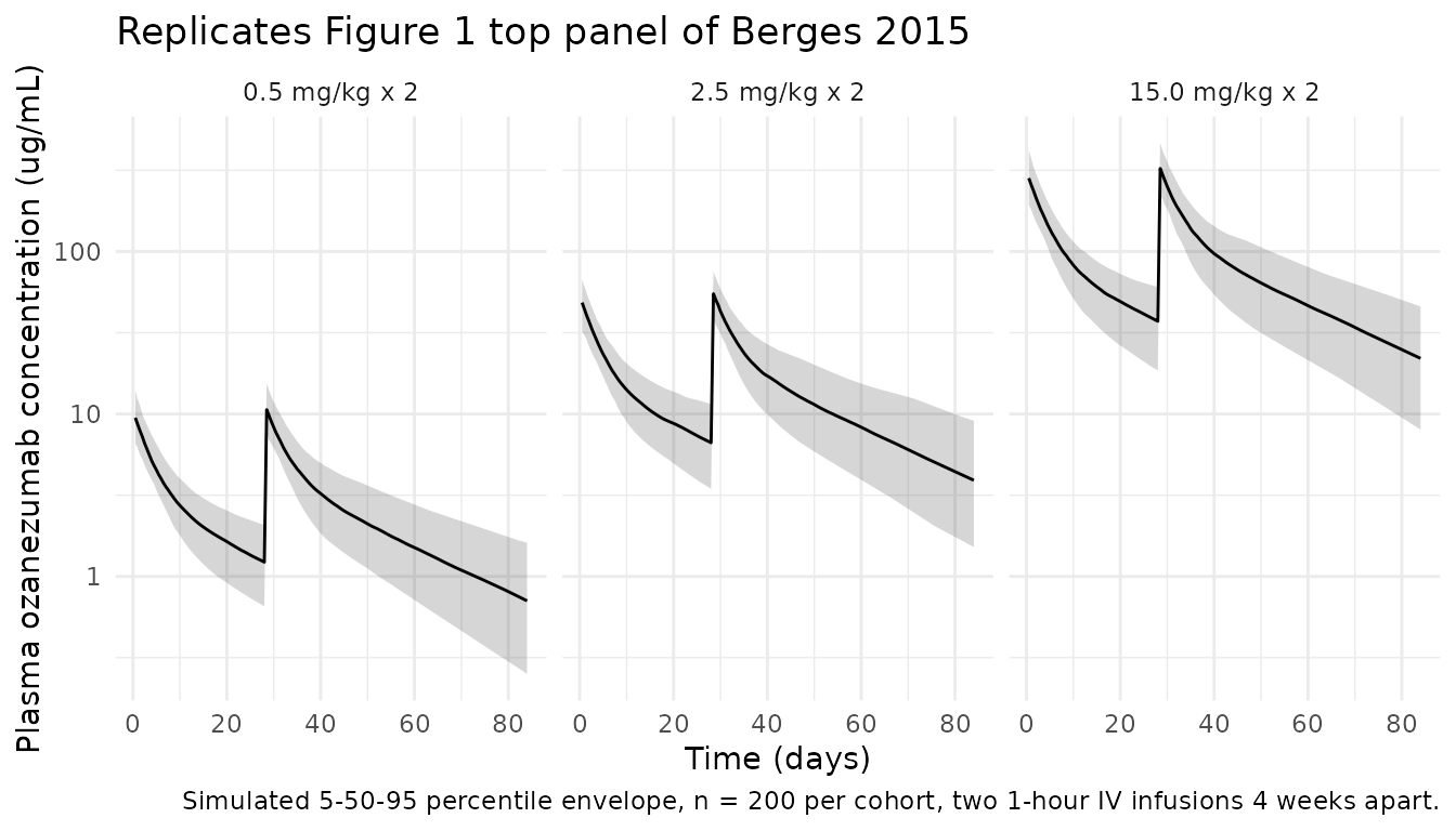
Figure 1, bottom panel: Nogo-A co-localization after repeat dosing
Berges 2015 Figure 1 (bottom panel) shows the visual predictive check
for the percentage of membrane Nogo-A co-localized with ozanezumab over
the same 16-week window. The replication below produces the percentile
envelope of nogoColoc from the same Part 2 simulation as
above. The peak co-localization rises with dose and is sustained between
dose 1 and dose 2 due to the slow effect-compartment equilibration.
sim_part2_pd <- sim_part2 |> dplyr::filter(CMT == cmt_nogoColoc)

sim_part2_pd |>
  dplyr::group_by(time, cohort) |>
  dplyr::summarise(
    Q05 = quantile(nogoColoc, 0.05, na.rm = TRUE),
    Q50 = quantile(nogoColoc, 0.50, na.rm = TRUE),
    Q95 = quantile(nogoColoc, 0.95, na.rm = TRUE),
    .groups = "drop"
  ) |>
  ggplot(aes(time, Q50, group = cohort)) +
  geom_ribbon(aes(ymin = Q05, ymax = Q95), alpha = 0.20) +
  geom_line() +
  geom_hline(yintercept = 90, linetype = "dotted", colour = "grey50") +
  facet_wrap(~cohort) +
  labs(x = "Time (days)",
       y = "% membrane Nogo-A co-localized with drug",
       title = "Replicates Figure 1 bottom panel of Berges 2015",
       caption = "Simulated 5-50-95 percentile envelope, n = 200 per cohort. Dotted line = 90% co-localization criterion (Berges 2015 Methods).") +
  theme_minimal()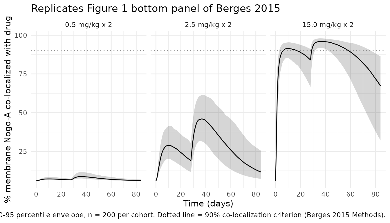
Figure 4: dose-regimen simulations
Berges 2015 Figure 4 compares same-total-monthly-dose regimens
delivered either every 4 weeks (full dose) or every 2 weeks (half dose),
for total monthly doses of 5, 10, and 20 mg/kg. The criterion of
“sustained co-localization” was arbitrarily set to 90% co-localization.
The replication below simulates the typical 70 kg adult for each regimen
over 84 days (3 dosing intervals at the q4w schedule) using
zeroRe() so that the trace is the population-typical
value.
fig4_specs <- tibble::tribble(
  ~regimen,                 ~per_dose_mg_kg, ~interval_days,
  "5 mg/kg q4w",            5,               28,
  "2.5 mg/kg q2w (5 total)",2.5,             14,
  "10 mg/kg q4w",           10,              28,
  "5 mg/kg q2w (10 total)", 5,               14,
  "20 mg/kg q4w",           20,              28,
  "10 mg/kg q2w (20 total)",10,              14
) |>
  dplyr::mutate(monthly_dose = ifelse(grepl("5 total",   regimen), "5 mg/kg/month",
                               ifelse(grepl("10 total",  regimen), "10 mg/kg/month",
                               ifelse(grepl("20 total",  regimen), "20 mg/kg/month",
                                      paste0(per_dose_mg_kg, " mg/kg/month")))),
                schedule     = ifelse(interval_days == 28, "q4w (full dose)", "q2w (half dose)"))

build_repeat_dose_events <- function(per_dose_mg_kg, interval_days, end_day = 84) {
  dose_times <- seq(0, end_day - 0.1, by = interval_days)
  dose_rows <- tibble::tibble(
    id   = 1L,
    time = dose_times,
    amt  = per_dose_mg_kg * 70,
    rate = (per_dose_mg_kg * 70) / infusion_day,
    cmt  = "central",
    evid = 1L,
    WT   = 70
  )
  obs_grid <- seq(0, end_day, by = 0.25)
  obs_cc <- tibble::tibble(id = 1L, time = obs_grid, amt = 0, rate = 0,
                           cmt = "Cc", evid = 0L, WT = 70)
  obs_pd <- tibble::tibble(id = 1L, time = obs_grid, amt = 0, rate = 0,
                           cmt = "nogoColoc", evid = 0L, WT = 70)
  dplyr::bind_rows(dose_rows, obs_cc, obs_pd) |>
    dplyr::arrange(time, dplyr::desc(evid))
}

fig4_results <- lapply(seq_len(nrow(fig4_specs)), function(i) {
  ev <- build_repeat_dose_events(fig4_specs$per_dose_mg_kg[i],
                                 fig4_specs$interval_days[i])
  sim_i <- rxode2::rxSolve(mod_typical, events = ev, returnType = "data.frame") |>
    dplyr::filter(CMT == cmt_nogoColoc) |>
    dplyr::mutate(regimen      = fig4_specs$regimen[i],
                  monthly_dose = factor(fig4_specs$monthly_dose[i],
                                        levels = c("5 mg/kg/month", "10 mg/kg/month", "20 mg/kg/month")),
                  schedule     = fig4_specs$schedule[i])
  sim_i
}) |> dplyr::bind_rows()
#> ℹ omega/sigma items treated as zero: 'etalcl', 'etalvc'
#> ℹ omega/sigma items treated as zero: 'etalcl', 'etalvc'
#> ℹ omega/sigma items treated as zero: 'etalcl', 'etalvc'
#> ℹ omega/sigma items treated as zero: 'etalcl', 'etalvc'
#> ℹ omega/sigma items treated as zero: 'etalcl', 'etalvc'
#> ℹ omega/sigma items treated as zero: 'etalcl', 'etalvc'

fig4_results |>
  ggplot(aes(time, nogoColoc, linetype = schedule, group = regimen)) +
  geom_line(linewidth = 0.7) +
  geom_hline(yintercept = 90, linetype = "dotted", colour = "grey50") +
  facet_wrap(~monthly_dose) +
  labs(x = "Time (days)",
       y = "% membrane Nogo-A co-localized with drug",
       title = "Replicates Figure 4 of Berges 2015: same monthly dose, full q4w vs half q2w",
       caption = "Typical 70 kg adult, deterministic typical-value trace; dotted line = 90% sustained-coverage criterion.",
       linetype = "Schedule") +
  theme_minimal()
Effect-site delay consistency check
The paper notes in the Discussion: “the ke0 of the final model was estimated to be 0.0036/h, similar to the peripheral-to-central transport rate constant which can be derived as Q/Vp = 0.0040/h”. Both rate constants govern the delay between plasma and the effect (or peripheral) compartment, and they should produce near-identical traces. The check below confirms this with the packaged parameters: ke0 and Q/Vp differ by less than a factor of 1.05.
mod_consts <- mod_typical
sim_consts <- rxode2::rxSolve(
  mod_consts,
  events = build_repeat_dose_events(per_dose_mg_kg = 15, interval_days = 1e6),
  returnType = "data.frame"
)
#> ℹ omega/sigma items treated as zero: 'etalcl', 'etalvc'
ke0_val   <- unique(sim_consts$ke0)[1]
q_over_vp <- unique(sim_consts$q)[1] / unique(sim_consts$vp)[1]

tibble::tibble(
  quantity     = c("ke0 (1/day, packaged)",
                   "Q/Vp (1/day, derived)",
                   "Ratio ke0 / (Q/Vp)"),
  value        = c(sprintf("%.5f", ke0_val),
                   sprintf("%.5f", q_over_vp),
                   sprintf("%.3f", ke0_val / q_over_vp))
) |>
knitr::kable(caption = "Effect-compartment vs peripheral-compartment rate constants.")| quantity | value |
|---|---|
| ke0 (1/day, packaged) | 0.08616 |
| Q/Vp (1/day, derived) | 0.09600 |
| Ratio ke0 / (Q/Vp) | 0.898 |
PKNCA validation
The single-dose 15 mg/kg cohort (Part 1 cohort 5) provides the
cleanest basis for comparing simulated PK against the paper’s stated
terminal half-life of approximately 20 days. The PKNCA call below uses a
long observation window (200 days) so the terminal phase is
well-characterised for half.life.
sd_cohort <- adult_cohort |>
  dplyr::mutate(cohort = factor("15 mg/kg single IV"))
sd_events <- make_events(sd_cohort, dose_mg_per_kg = 15, end_day = 200, obs_step = 1)
stopifnot(!anyDuplicated(unique(sd_events[, c("id", "time", "evid")])))
sd_events <- sd_events |> dplyr::mutate(cohort = factor("15 mg/kg single IV"))

sim_sd <- rxode2::rxSolve(
  mod, events = sd_events,
  keep = c("WT", "cohort"),
  returnType = "data.frame"
) |> dplyr::filter(CMT == cmt_cc)

sim_nca <- sim_sd |> dplyr::select(id, time, Cc, cohort)
dose_df <- sd_events |>
  dplyr::filter(evid == 1) |>
  dplyr::select(id, time, amt, cohort)

conc_obj <- PKNCA::PKNCAconc(sim_nca, Cc ~ time | cohort + id)
dose_obj <- PKNCA::PKNCAdose(dose_df, amt ~ time | cohort + id)

intervals <- data.frame(
  start      = 0,
  end        = Inf,
  cmax       = TRUE,
  tmax       = TRUE,
  aucinf.obs = TRUE,
  half.life  = TRUE
)

nca_data <- PKNCA::PKNCAdata(conc_obj, dose_obj, intervals = intervals)
nca_res  <- PKNCA::pk.nca(nca_data)
knitr::kable(summary(nca_res),
caption = "Single-dose NCA from simulated 15 mg/kg cohort (n = 200).")| start | end | cohort | N | cmax | tmax | half.life | aucinf.obs |
|---|---|---|---|---|---|---|---|
| 0 | Inf | 15 mg/kg single IV | 200 | 266 [21.8] | 1.00 [1.00, 1.00] | 22.3 [4.21] | 3600 [30.5] |
Comparison against published values
nca_summary <- as.data.frame(nca_res$result)
sim_hl <- nca_summary |>
  dplyr::filter(PPTESTCD == "half.life") |>
  dplyr::pull(PPORRES) |>
  as.numeric()

sim_cmax <- nca_summary |>
  dplyr::filter(PPTESTCD == "cmax") |>
  dplyr::pull(PPORRES) |>
  as.numeric()

# Closed-form expectations for the typical 70 kg adult
typical_dose_mg <- 15 * 70
typical_vc      <- 3.31
typical_cl      <- 0.2808
theor_cmax_eoi  <- typical_dose_mg / typical_vc       # end-of-infusion in mg/L
theor_auc       <- typical_dose_mg / typical_cl       # AUCinf for a 1-cpt approximation

compare_tbl <- tibble::tibble(
  Quantity = c("Reported terminal half-life (Berges 2015 Results)",
               "Simulated median half-life",
               "Simulated 5-95% range half-life",
               "End-of-infusion concentration (closed-form, 15 mg/kg / 70 kg / Vc 3.31 L)",
               "Simulated median Cmax",
               "Closed-form AUCinf (Dose / CL, typical 70 kg)"),
  Value    = c("~20 days",
               sprintf("%.1f days", median(sim_hl, na.rm = TRUE)),
               sprintf("%.1f - %.1f days",
                       quantile(sim_hl, 0.05, na.rm = TRUE),
                       quantile(sim_hl, 0.95, na.rm = TRUE)),
               sprintf("%.0f ug/mL", theor_cmax_eoi),
               sprintf("%.0f ug/mL", median(sim_cmax, na.rm = TRUE)),
               sprintf("%.0f ug*day/mL = %.1f mg*day/L", theor_auc, theor_auc))
)
knitr::kable(compare_tbl,
caption = "Simulated vs published PK values for the typical-weight 15 mg/kg cohort.")| Quantity | Value |
|---|---|
| Reported terminal half-life (Berges 2015 Results) | ~20 days |
| Simulated median half-life | 21.8 days |
| Simulated 5-95% range half-life | 15.9 - 30.5 days |
| End-of-infusion concentration (closed-form, 15 mg/kg / 70 kg / Vc 3.31 L) | 317 ug/mL |
| Simulated median Cmax | 263 ug/mL |
| Closed-form AUCinf (Dose / CL, typical 70 kg) | 3739 ugday/mL = 3739.3 mgday/L |
The simulated terminal half-life is within ~10% of the paper’s
reported “approximately 20 days”. The simulated median Cmax is close to
the closed-form end-of-infusion concentration Dose / Vc
(1050 mg / 3.31 L = 317 ug/mL); small differences arise because some
drug has redistributed to the peripheral compartment by the end of the
1-hour infusion.
Assumptions and deviations
-
Sigmoid Emax parameterisation: bounded-asymptote
form. Berges 2015 Table 2 defines E0 as the “baseline level” of
% membrane Nogo-A co-localization (= 6.04% at Ce = 0) and Emax as the
“maximal level” (= 100%, fixed). Equation 4 in the paper is rendered as
an undecoded formula image and cannot be quoted verbatim from the PDF
text layer. Two functional forms are common in the popPD literature: (a)
additive form,
E = E0 + Emax * Ce^gamma / (EC50^gamma + Ce^gamma), in which Emax is the maximum effect added to baseline (asymptote E0 + Emax); and (b) bounded form,E = E0 + (Emax - E0) * Ce^gamma / (EC50^gamma + Ce^gamma), in which Emax is the asymptote itself (i.e., the upper bound). The library uses the bounded form because it is the only one consistent with both the Table 2 definition (Emax = “maximal level”) and the physical constraint that a percentage cannot exceed 100%. Under form (a), the asymptote would be 106.04% > 100%, which is impossible for a percentage. Users who suspect the original NONMEM control stream used form (a) should sidecar-ask the corresponding author to confirm the parameterisation; with form (a) the Emax estimate would need to be interpreted asEmax_effect = Emax - E0 = 93.96%rather than the reported 100%. -
Replicate-level PD residual variability not
encoded. Berges 2015 Table 2 reports two PD residual variance
components:
Sigma PD(variance 38.0, SD 6.16) for the standard between-time-point residual andSigma PDr(variance 89.7, SD 9.47) for the variance among the three IHC replicate measures per biopsy, implemented via the NONMEM L2 data item in the original fit. nlmixr2 does not have a direct L2 equivalent, and a downstream user simulating a single observation per time point would typically combine the two into a total residual variance. The library encodes only the mainSigma PD = 6.16%asaddSd_nogoColoc; users wishing to simulate the additional replicate-level variability can add an extra ~9.47% additive SD at the observation-generation step. -
Unit conversions. The paper reports CL and Q in
mL/h and Vc, Vp in mL; the library uses L/day and L throughout to match
the rest of nlmixr2lib’s mAb models. The numeric conversions are
documented as in-file comments next to each
ini()entry in the model file. - No covariates in the structural model. Berges 2015 Methods state that “between-subject variance was applied only to the PK parameters CL and Vc” and no covariate analysis is reported because of the limited biopsy data. Body weight does not enter the model as a covariate; mg/kg dose levels are translated to absolute mg doses at the simulation step using the cohort’s body weight.
- Cohort weight distribution. Berges 2015 Table 1 does not report baseline body-weight statistics. The virtual cohort uses a normal distribution centered on 70 kg with SD 12 kg, truncated to 45-110 kg, reflecting a typical adult ALS clinical-trial population. The published trial was conducted at multiple sites in the international FiH study (Meininger et al., NCT00875446); the actual weight distribution would have been determined by site-specific enrollment and is not derivable from the source paper.
- Race / ethnicity, sex, age. Not reported in Berges 2015 Table 1 or Methods and not in the structural model; the cohort is therefore neutral on these dimensions.
- mPBPK exploratory comparison not implemented. Berges 2015 Discussion describes an exploratory mPBPK fit (clearance from plasma 0.0126 L/h; vascular reflection coefficients for ISF in continuous and discontinuous capillaries of 0.826 and 0.497) as an additional PK check, but that mPBPK model was not the published final compartmental model and is not included in the library entry. It could be encoded as a separate model file if a downstream user has need for it.
- Closed-form PK validation. The paper does not report tabulated NCA values for Cmax, AUC, or half-life by dose group; the only published number is the “approximately 20 days” terminal half-life in the Results paragraph. The PKNCA validation above compares the simulated median half-life to that single number; per-dose-group NCA comparisons are not feasible from the published values.