Ceftolozane + tazobactam plasma and epithelial lining fluid (Zhang 2021)
Source:vignettes/articles/Zhang_2021_ceftolozane_tazobactam.Rmd
Zhang_2021_ceftolozane_tazobactam.RmdModel and source
Zhang 2021 updated the ceftolozane and tazobactam population PK models of Chandorkar 2015 with data from 16 studies, including the phase 3 ASPECT-NP trial in ventilated patients with hospital-acquired or ventilator-associated pneumonia, and added a link model for epithelial lining fluid (ELF). The two analytes were fitted as separate models, so they are packaged as two model files sharing this one vignette:
-
Zhang_2021_ceftolozaneandZhang_2021_tazobactam: two-compartment plasma models with zero-order (1-hour infusion) input and first-order elimination, plus a hypothetical ELF link compartment. - Article: https://doi.org/10.1002/jcph.1733 (PMC7821292, open access).
- Supplement: Supplemental Tables S1-S2 (studies, sites) and
Supplemental Figures S1-S3. Figure S1 prints the ODEs of the three ELF
structures tested; model 3, the selected one, is
dA3/dt = K1E * A1 - KE0 * A3with noA3term indA1/dtand the ELF volumeV3equal toV1.
ui_cef <- rxode2::rxode(readModelDb("Zhang_2021_ceftolozane"))
#> ℹ parameter labels from comments will be replaced by 'label()'
#> Warning: some etas defaulted to non-mu referenced, possible parsing error: etalk_central_elf, etalk_central_elf_pneumonia
#> as a work-around try putting the mu-referenced expression on a simple line
ui_taz <- rxode2::rxode(readModelDb("Zhang_2021_tazobactam"))
#> ℹ parameter labels from comments will be replaced by 'label()'
#> Warning: some etas defaulted to non-mu referenced, possible parsing error: etalk_central_elf, etalk_central_elf_pneumonia
#> as a work-around try putting the mu-referenced expression on a simple line

cat(ui_cef$description, "\n\n")
#> Two-compartment population PK model for ceftolozane given as a 1-hour intravenous infusion (alone or with tazobactam), fitted to 8,330 plasma concentrations from 968 adults pooled across 16 studies, including 305 ventilated patients with hospital-acquired or ventilator-associated pneumonia from the phase 3 ASPECT-NP trial (Zhang 2021). Elimination is first order. Baseline Cockcroft-Gault creatinine clearance acts on clearance through a power function, with an additional end-stage renal disease factor; body weight acts on both volumes through estimated power exponents; infection type (cUTI, cIAI, pneumonia, other infection) shifts clearance and central volume against a healthy-participant reference. Correlated IIV on CL and Vc, independent IIV on Vp. A hypothetical epithelial-lining-fluid (ELF) link compartment without mass transfer (influx K1E from the central amount, elimination KE0, ELF volume equal to Vc) predicts ELF concentrations; pneumonia lowers K1E and KE0 by one shared factor and IIV on K1E differs between healthy participants and pneumonia patients. Companion model to Zhang_2021_tazobactam, fitted separately in the same paper.
cat(ui_taz$description, "\n")
#> Two-compartment population PK model for tazobactam given as a 1-hour intravenous infusion (alone or with ceftolozane), fitted to 5,679 plasma concentrations from 835 adults pooled across 16 studies, including 305 ventilated patients with hospital-acquired or ventilator-associated pneumonia from the phase 3 ASPECT-NP trial (Zhang 2021). Elimination is first order. Baseline Cockcroft-Gault creatinine clearance acts on clearance through a power function, with an additional end-stage renal disease factor on clearance and central volume; body weight acts on both volumes through estimated power exponents; infection type (cIAI, pneumonia, other infection on Vc; cUTI, cIAI, pneumonia on Vp) shifts the volumes against a healthy-participant reference. Correlated IIV on CL and Vc, independent IIV on Vp. A hypothetical epithelial-lining-fluid (ELF) link compartment without mass transfer (influx K1E from the central amount, elimination KE0, ELF volume equal to Vc) predicts ELF concentrations; pneumonia lowers K1E and KE0 by one shared factor and IIV on K1E differs between healthy participants and pneumonia patients. Companion model to Zhang_2021_ceftolozane, fitted separately in the same paper.
How the ELF link model works
Because the link compartment does not deplete plasma and its volume
equals the central volume, its concentration obeys
dCelf/dt = K1E * Cc - KE0 * Celf. Two consequences follow
and are gated below:
- at steady state the ELF-to-plasma AUC ratio over a dosing interval
is exactly
K1E / KE0for every subject; - pneumonia multiplies K1E and KE0 by the same factor (0.0339 for ceftolozane, 0.479 for tazobactam; Table 3), so it slows ELF equilibration without changing that ratio.
Population
The plasma data set holds 8,330 ceftolozane observations from 968 adults and 5,679 tazobactam observations from 835 adults (Methods, Table 1). Of these, 305 are ASPECT-NP patients with ventilated nosocomial pneumonia. The ceftolozane population was 60.2% male, mean age 53.2 years (range 18-98), mean weight 74.7 kg (range 33.5-173) and mean Cockcroft-Gault creatinine clearance 109.9 mL/min (range 6.3-531.3). Infection type was healthy (28.6%, including renal impairment without infection), cUTI (18.2%), cIAI (18.0%), pneumonia (34.2%) or other infection (1.0%, critically ill patients with augmented renal clearance). ASPECT-NP patients averaged 81.5 kg and 124.1 mL/min.
ELF was sampled once per participant by bronchoalveolar lavage at 1, 2, 4, 6 or 8 hours after the start of infusion in two phase 1 studies (Supplemental Table S1): CXA-ELF-10-03 (healthy volunteers, three doses of 1 g/0.5 g q8h) and CXA-ICU-14-01 group 1 (mechanically ventilated patients with proven or suspected pneumonia, 2 g/1 g q8h for 4-6 doses), giving 47 ceftolozane and 42 tazobactam ELF observations.
The same information is in each model’s population
metadata.
Source trace
| Quantity | Ceftolozane | Tazobactam | Source |
|---|---|---|---|
| CL at CrCL 100 mL/min (L/h) | 4.84 | 16.6 | Table 2 |
| CrCL/100 exponent on CL | 0.701 | 0.623 | Table 2 |
| ESRD factor on CL | 0.320 | 0.626 | Table 2 |
| cUTI / cIAI factor on CL | 1.18 / 1.43 | - | Table 2 |
| Vc at 70 kg (L) | 9.23 | 13.1 | Table 2 |
| WT/70 exponent on Vc | 0.684 | 0.629 | Table 2 |
| cUTI / cIAI / pneumonia / other factor on Vc | 1.25 / 1.59 / 2.00 / 2.14 | - / 1.49 / 2.17 / 2.49 | Table 2 |
| ESRD factor on Vc | 1.30 | 0.749 | Table 2 |
| Q (L/h) | 3.13 | 4.05 | Table 2 |
| Vp at 70 kg (L) | 4.78 | 4.89 | Table 2 |
| WT/70 exponent on Vp | 0.484 | 0.530 | Table 2 |
| cUTI / cIAI / pneumonia factor on Vp | - | 1.25 / 1.34 / 2.06 | Table 2 |
| IIV CL, Vc, Vp (%CV); cov(CL, Vc) | 36.1, 42.9, 15.1; 0.073 | 53.1, 38.7, 19.4; 0.071 | Table 2 |
| Residual error (sigma^2) | prop 0.0248, add 0.00984 | prop 0.081 | Table 2 and footnote d |
| K1E, KE0 healthy (1/h) | 0.808, 1.56 | 0.262, 0.691 | Table 3 |
| Pneumonia factor on K1E and KE0 | 0.0339 | 0.479 | Table 3 equations |
| IIV K1E healthy / pneumonia (%CV) | 39.6 / 81.2 | 65.5 / 84.4 | Table 3 |
| ELF residual error (sigma^2) | prop 0.0249, add 0.00834 | prop 0.055 | Table 3 and footnote d |
| Covariate equations | CL, Vc, Vp | CL, Vc, Vp | Equations under Table 2 |
| ELF ODE, V3 = V1 | model 3 | model 3 | Supplemental Figure S1 |
Two scale choices are fixed from the paper’s own numbers rather than assumed:
-
IIV. The %CV column is
sqrt(omega^2) * 100. Table 2 footnote c gives the ceftolozane CL-Vc correlation as r = 0.474 next to cov = 0.073. That value is reproduced by omega^2 = CV^2 (r = 0.471) and not by omega^2 = log(1 + CV^2) (r = 0.507). -
Residual error. The printed RV values are
variances. Footnote d prints the plasma %CV as
sqrt(F^2 * 0.0248 + 0.00984) / F * 100, which gives the printed “100%-15.7% CV” across F = 0.1-200 ug/mL.
om <- ui_cef$omega
r_cl_vc <- om["etalcl", "etalvc"] / sqrt(om["etalcl", "etalcl"] * om["etalvc", "etalvc"])

rv_cv <- function(f, prop, add = 0) 100 * sqrt(f^2 * prop^2 + add^2) / f
p_cef <- ui_cef$theta
p_taz <- ui_taz$theta

scale_tab <- tibble::tribble(
  ~quantity, ~model, ~paper,
  "Ceftolozane r(CL, Vc)", r_cl_vc, 0.474,
  "Ceftolozane plasma RV %CV at 0.1 ug/mL", rv_cv(0.1, p_cef[["propSd"]], p_cef[["addSd"]]), 100,
  "Ceftolozane plasma RV %CV at 200 ug/mL", rv_cv(200, p_cef[["propSd"]], p_cef[["addSd"]]), 15.7,
  "Ceftolozane ELF RV %CV at 0.1 ug/mL", rv_cv(0.1, p_cef[["propSd_Celf"]], p_cef[["addSd_Celf"]]), 92.7,
  "Ceftolozane ELF RV %CV at 100 ug/mL", rv_cv(100, p_cef[["propSd_Celf"]], p_cef[["addSd_Celf"]]), 15.8,
  "Tazobactam plasma RV %CV", rv_cv(1, p_taz[["propSd"]]), 28.5,
  "Tazobactam ELF RV %CV", rv_cv(1, p_taz[["propSd_Celf"]]), 23.4
)
scale_tab |>
  dplyr::mutate(model = signif(model, 4)) |>
  dplyr::rename("Quantity" = quantity, "Model" = model, "Paper" = paper) |>
knitr::kable()| Quantity | Model | Paper |
|---|---|---|
| Ceftolozane r(CL, Vc) | 0.4714 | 0.474 |
| Ceftolozane plasma RV %CV at 0.1 ug/mL | 100.4000 | 100.000 |
| Ceftolozane plasma RV %CV at 200 ug/mL | 15.7500 | 15.700 |
| Ceftolozane ELF RV %CV at 0.1 ug/mL | 92.6800 | 92.700 |
| Ceftolozane ELF RV %CV at 100 ug/mL | 15.7800 | 15.800 |
| Tazobactam plasma RV %CV | 28.4600 | 28.500 |
| Tazobactam ELF RV %CV | 23.4500 | 23.400 |
# Deterministic: both columns come from the same printed values; the only
# slack is the rounding of the printed digits (3 significant figures, and the
# '100%' end of the plasma range is 100.4% before rounding).
stopifnot(
  abs(r_cl_vc - 0.474) < 0.005,
  all(abs(scale_tab$model[-1] - scale_tab$paper[-1]) < 0.05 + 0.005 * scale_tab$paper[-1])
)
Reproducing the paper’s covariate statements
The Results, Discussion and Conclusions translate the covariate
effects into percentages. Each is checked below by solving the packaged
model at typical values (random effects zeroed) and reading the
individual parameters back out, which exercises the full
ini() to model() wiring rather than re-doing
the arithmetic by hand.
# Scenario rows share CrCL 100 mL/min and 70 kg; only the indicator changes.
base_cov <- tibble::tibble(
  CRCL = 100, WT = 70, RENALIMP_ESRD = 0, DIS_CUTI = 0, DIS_CIAI = 0,
  DIS_PNEUMONIA = 0, DIS_OTHER_INFECT = 0
)
scenarios <- dplyr::bind_rows(
  base_cov |> dplyr::mutate(scenario = "Healthy"),
  base_cov |> dplyr::mutate(scenario = "ESRD", RENALIMP_ESRD = 1),
  base_cov |> dplyr::mutate(scenario = "cUTI", DIS_CUTI = 1),
  base_cov |> dplyr::mutate(scenario = "cIAI", DIS_CIAI = 1),
  base_cov |> dplyr::mutate(scenario = "Pneumonia", DIS_PNEUMONIA = 1),
  base_cov |> dplyr::mutate(scenario = "Other infection", DIS_OTHER_INFECT = 1)
) |>
  dplyr::mutate(id = dplyr::row_number())
cov_cols <- setdiff(names(base_cov), character(0))

typical_params <- function(ui) {
  ev <- dplyr::bind_rows(
    scenarios |> dplyr::mutate(time = 0, amt = 1000, rate = 1000, evid = 1L,
                               cmt = "central", dvid = NA_integer_),
    scenarios |> dplyr::mutate(time = 1, amt = NA_real_, rate = NA_real_,
                               evid = 0L, cmt = NA_character_, dvid = 1L)
  ) |>
    dplyr::arrange(id, time, dplyr::desc(evid))
  rxode2::rxSolve(rxode2::zeroRe(ui), events = ev, omega = NA, sigma = NA,
                  keep = "scenario", returnType = "data.frame") |>
    dplyr::filter(time == 1) |>
    dplyr::select(scenario, cl, vc, vp, k_central_elf, ke0)
}
tp_cef <- typical_params(ui_cef)
#> Warning: some etas defaulted to non-mu referenced, possible parsing error: etalk_central_elf, etalk_central_elf_pneumonia
#> as a work-around try putting the mu-referenced expression on a simple line
tp_taz <- typical_params(ui_taz)
#> Warning: some etas defaulted to non-mu referenced, possible parsing error: etalk_central_elf, etalk_central_elf_pneumonia
#> as a work-around try putting the mu-referenced expression on a simple line

rel <- function(tp, scen, par) {
  tp[[par]][tp$scenario == scen] / tp[[par]][tp$scenario == "Healthy"]
}

statements <- tibble::tribble(
  ~statement, ~model, ~paper,
  "Ceftolozane CL, ESRD: '68% lower'", 100 * (1 - rel(tp_cef, "ESRD", "cl")), 68,
  "Ceftolozane Vc, ESRD: '30.0% higher'", 100 * (rel(tp_cef, "ESRD", "vc") - 1), 30.0,
  "Ceftolozane Vc, pneumonia: '100% increase'", 100 * (rel(tp_cef, "Pneumonia", "vc") - 1), 100,
  "Tazobactam CL, ESRD: '37.4% lower'", 100 * (1 - rel(tp_taz, "ESRD", "cl")), 37.4,
  "Tazobactam Vc, ESRD: '25.1% lower'", 100 * (1 - rel(tp_taz, "ESRD", "vc")), 25.1,
  "Tazobactam Vc, pneumonia: '117% higher'", 100 * (rel(tp_taz, "Pneumonia", "vc") - 1), 117,
  "Tazobactam Vp, pneumonia: '106%' higher", 100 * (rel(tp_taz, "Pneumonia", "vp") - 1), 106,
  "Tazobactam Vp, cUTI: '25%' higher", 100 * (rel(tp_taz, "cUTI", "vp") - 1), 25,
  "Tazobactam Vp, cIAI: '34%' higher", 100 * (rel(tp_taz, "cIAI", "vp") - 1), 34,
  "Ceftolozane K1E, pneumonia: 'approximately 97% lower'", 100 * (1 - rel(tp_cef, "Pneumonia", "k_central_elf")), 97,
  "Ceftolozane KE0, pneumonia: 'approximately 97% lower'", 100 * (1 - rel(tp_cef, "Pneumonia", "ke0")), 97,
  "Tazobactam K1E, pneumonia: '52% lower'", 100 * (1 - rel(tp_taz, "Pneumonia", "k_central_elf")), 52,
  "Tazobactam KE0, pneumonia: '52% lower'", 100 * (1 - rel(tp_taz, "Pneumonia", "ke0")), 52,
  "Ceftolozane typical K1E (1/h): '0.808'", tp_cef$k_central_elf[tp_cef$scenario == "Healthy"], 0.808,
  "Ceftolozane typical KE0 (1/h): '1.56'", tp_cef$ke0[tp_cef$scenario == "Healthy"], 1.56,
  "Tazobactam typical K1E (1/h): '0.262'", tp_taz$k_central_elf[tp_taz$scenario == "Healthy"], 0.262,
  "Tazobactam typical KE0 (1/h): '0.691'", tp_taz$ke0[tp_taz$scenario == "Healthy"], 0.691
)
statements |>
  dplyr::mutate(model = signif(model, 4)) |>
  dplyr::rename("Paper statement" = statement, "Model" = model, "Paper" = paper) |>
knitr::kable()| Paper statement | Model | Paper |
|---|---|---|
| Ceftolozane CL, ESRD: ‘68% lower’ | 68.000 | 68.000 |
| Ceftolozane Vc, ESRD: ‘30.0% higher’ | 30.000 | 30.000 |
| Ceftolozane Vc, pneumonia: ‘100% increase’ | 100.000 | 100.000 |
| Tazobactam CL, ESRD: ‘37.4% lower’ | 37.400 | 37.400 |
| Tazobactam Vc, ESRD: ‘25.1% lower’ | 25.100 | 25.100 |
| Tazobactam Vc, pneumonia: ‘117% higher’ | 117.000 | 117.000 |
| Tazobactam Vp, pneumonia: ‘106%’ higher | 106.000 | 106.000 |
| Tazobactam Vp, cUTI: ‘25%’ higher | 25.000 | 25.000 |
| Tazobactam Vp, cIAI: ‘34%’ higher | 34.000 | 34.000 |
| Ceftolozane K1E, pneumonia: ‘approximately 97% lower’ | 96.610 | 97.000 |
| Ceftolozane KE0, pneumonia: ‘approximately 97% lower’ | 96.610 | 97.000 |
| Tazobactam K1E, pneumonia: ‘52% lower’ | 52.100 | 52.000 |
| Tazobactam KE0, pneumonia: ‘52% lower’ | 52.100 | 52.000 |
| Ceftolozane typical K1E (1/h): ‘0.808’ | 0.808 | 0.808 |
| Ceftolozane typical KE0 (1/h): ‘1.56’ | 1.560 | 1.560 |
| Tazobactam typical K1E (1/h): ‘0.262’ | 0.262 | 0.262 |
| Tazobactam typical KE0 (1/h): ‘0.691’ | 0.691 | 0.691 |
# Deterministic: the paper quotes these to 2-3 significant digits, so a
# 0.6-point absolute (or 0.5% relative) band is the rounding floor. A wrong
# factor, a dropped indicator or a sign error misses by tens of points.
stopifnot(
  all(abs(statements$model - statements$paper) <= pmax(0.6, 0.005 * statements$paper))
)
Virtual cohorts
Observed data are not available. Three cohorts approximate the populations behind the paper’s concentration-time figures:
- ASPECT-NP pneumonia patients (Figure 1): weight normal about the ASPECT-NP mean 81.5 kg (SD 17.4) within the observed 42-150.1 kg; CrCL log-normal with the ASPECT-NP mean 124.1 mL/min and SD 70.3 within the observed 14.9-531.3 mL/min. Dose follows the trial’s renal bands: 2 g/1 g for CrCL > 50 mL/min, 1 g/0.5 g for 30-50 and 0.5 g/0.25 g below 30. Twenty q8h doses, so the last interval is at steady state.
- Healthy ELF volunteers (Figure 4A-B): three 1 g/0.5 g doses q8h, ELF profile after the third dose. The paper does not print this subgroup’s demographics; weight normal 75 kg (SD 12, 50-110 kg) and CrCL log-normal about 115 mL/min (CV 20%, 80-180 mL/min) are assumed.
- Ventilated ICU pneumonia patients (Figure 4C-D): 2 g/1 g q8h, ELF profile after the fifth dose (the study gave 4-6); covariates drawn as for the ASPECT-NP cohort.
A band limit is part of a cohort’s definition, so out-of-band draws are rejected and redrawn rather than clamped.
# rxSetSeed() fixes rxode2's draw for a given build and thread count, not
# across them, so every assertion below is written on centres and robust
# quantiles rather than on cohort extremes.
set.seed(20210201)
rxode2::rxSetSeed(20210201)

N_PER_ARM <- 200L

draw_band <- function(n, draw, lo, hi) {
  out <- numeric(0)
  while (length(out) < n) {
    x <- draw(2L * n)
    out <- c(out, x[x >= lo & x <= hi])
  }
  out[seq_len(n)]
}
sdlog_np <- sqrt(log(1 + (70.3 / 124.1)^2))
meanlog_np <- log(124.1) - sdlog_np^2 / 2

make_subjects <- function(n, cohort, id_offset, pneumonia, wt, crcl) {
  tibble::tibble(
    id = id_offset + seq_len(n), cohort = cohort,
    CRCL = crcl, WT = wt, RENALIMP_ESRD = 0, DIS_CUTI = 0, DIS_CIAI = 0,
    DIS_PNEUMONIA = pneumonia, DIS_OTHER_INFECT = 0
  )
}

subj_np <- make_subjects(
  N_PER_ARM, "ASPECT-NP", 0L, 1,
  wt = draw_band(N_PER_ARM, function(k) rnorm(k, 81.5, 17.4), 42, 150.1),
  crcl = draw_band(N_PER_ARM, function(k) rlnorm(k, meanlog_np, sdlog_np), 14.9, 531.3)
) |>
  dplyr::mutate(dose_cef = dplyr::case_when(
    CRCL > 50 ~ 2000, CRCL >= 30 ~ 1000, TRUE ~ 500
  ))
subj_hv <- make_subjects(
  N_PER_ARM, "Healthy ELF", 1000L, 0,
  wt = draw_band(N_PER_ARM, function(k) rnorm(k, 75, 12), 50, 110),
  crcl = draw_band(N_PER_ARM, function(k) rlnorm(k, log(115), 0.2), 80, 180)
) |>
  dplyr::mutate(dose_cef = 1000)
subj_icu <- make_subjects(
  N_PER_ARM, "ICU pneumonia ELF", 2000L, 1,
  wt = draw_band(N_PER_ARM, function(k) rnorm(k, 81.5, 17.4), 42, 150.1),
  crcl = draw_band(N_PER_ARM, function(k) rlnorm(k, meanlog_np, sdlog_np), 14.9, 531.3)
) |>
  dplyr::mutate(dose_cef = 2000)

# Tazobactam is always given at half the ceftolozane dose (fixed 2:1 product).
subjects <- dplyr::bind_rows(subj_np, subj_hv, subj_icu) |>
  dplyr::mutate(dose_taz = dose_cef / 2)
stopifnot(!anyDuplicated(subjects$id))

design <- tibble::tribble(
  ~cohort,             ~n_dose, ~ii,
  "ASPECT-NP",         20L,     8,
  "Healthy ELF",       3L,      8,
  "ICU pneumonia ELF", 5L,      8
) |>
  dplyr::mutate(t_last = (n_dose - 1L) * ii)

# The model has two observed outputs (Cc and Celf), so observation rows are
# tagged by dvid with a blank cmt; both concentrations are returned on every
# observation row. Doses are 1-hour infusions into central (rate = amt / 1 h).
make_events <- function(dose_col) {
  subj <- subjects |>
    dplyr::inner_join(design, by = "cohort") |>
    dplyr::mutate(amt = .data[[dose_col]])
  doses <- subj |>
    dplyr::mutate(time = 0, rate = amt, addl = n_dose - 1L, evid = 1L,
                  cmt = "central", dvid = NA_integer_)
  grid <- c(seq(0, 1.5, by = 0.05), seq(1.75, 8, by = 0.25))
  obs <- subj |>
    tidyr::crossing(tad = grid) |>
    dplyr::mutate(time = t_last + tad, amt = NA_real_, rate = NA_real_,
                  addl = NA_integer_, evid = 0L, cmt = NA_character_, dvid = 1L) |>
    dplyr::select(-tad)
  dplyr::bind_rows(doses, obs) |>
    dplyr::select(id, time, amt, rate, ii, addl, evid, cmt, dvid, cohort,
                  dose_cef, dose_taz, t_last, CRCL, WT, RENALIMP_ESRD,
                  DIS_CUTI, DIS_CIAI, DIS_PNEUMONIA, DIS_OTHER_INFECT) |>
    dplyr::arrange(id, time, dplyr::desc(evid))
}
ev_cef <- make_events("dose_cef")
ev_taz <- make_events("dose_taz")
Simulation
solve_cohorts <- function(ui, ev) {
  rxode2::rxSolve(ui, events = ev, keep = c("cohort", "dose_cef", "dose_taz", "t_last"),
                  returnType = "data.frame") |>
    dplyr::mutate(tad = round(time - t_last, 2))
}
sim_cef <- solve_cohorts(ui_cef, ev_cef)
sim_taz <- solve_cohorts(ui_taz, ev_taz)

stopifnot(
  all(sim_cef$Cc >= 0), all(sim_cef$Celf >= 0),
  all(sim_taz$Cc >= 0), all(sim_taz$Celf >= 0),
  dplyr::n_distinct(sim_cef$id) == 3L * N_PER_ARM
)
Replicate published figures
The predicted-median lines of Figures 1 and 4 were digitized by the maintainers from the published raster images (axis ticks located to the pixel, then the middle of the three blue prediction lines read at each time). They are the paper’s own model predictions, so they are the right target for a packaged model; the observed-data medians depend on the unavailable data set.
fig1 <- tibble::tribble(
  ~drug,         ~tad, ~pred_median,
  "Ceftolozane", 1,    81.4,
  "Ceftolozane", 4,    40.9,
  "Ceftolozane", 6,    25.2,
  "Ceftolozane", 7,    22.2,
  "Ceftolozane", 8,    19.3,
  "Tazobactam",  1,    17.8,
  "Tazobactam",  2,    11.5,
  "Tazobactam",  4,    3.82,
  "Tazobactam",  5,    2.61,
  "Tazobactam",  7,    1.44,
  "Tazobactam",  8,    1.16
)
fig4 <- tibble::tribble(
  ~drug,         ~cohort,             ~tad, ~pred_median,
  "Ceftolozane", "Healthy ELF",       1,    20.0,
  "Ceftolozane", "Healthy ELF",       2.25, 23.5,
  "Ceftolozane", "Healthy ELF",       4,    11.0,
  "Ceftolozane", "Healthy ELF",       6,    4.93,
  "Tazobactam",  "Healthy ELF",       1,    2.13,
  "Tazobactam",  "Healthy ELF",       2.25, 2.56,
  "Tazobactam",  "Healthy ELF",       4,    1.04,
  "Tazobactam",  "Healthy ELF",       6,    0.368,
  "Tazobactam",  "Healthy ELF",       8,    0.173,
  "Ceftolozane", "ICU pneumonia ELF", 1,    16.6,
  "Ceftolozane", "ICU pneumonia ELF", 2.25, 15.6,
  "Ceftolozane", "ICU pneumonia ELF", 4,    21.4,
  "Ceftolozane", "ICU pneumonia ELF", 6,    20.0,
  "Ceftolozane", "ICU pneumonia ELF", 8,    17.5,
  "Tazobactam",  "ICU pneumonia ELF", 1,    3.11,
  "Tazobactam",  "ICU pneumonia ELF", 2.25, 3.32,
  "Tazobactam",  "ICU pneumonia ELF", 4,    4.01,
  "Tazobactam",  "ICU pneumonia ELF", 6,    2.78,
  "Tazobactam",  "ICU pneumonia ELF", 8,    1.58
)

sim_all <- dplyr::bind_rows(
  sim_cef |> dplyr::mutate(drug = "Ceftolozane"),
  sim_taz |> dplyr::mutate(drug = "Tazobactam")
)
pct <- sim_all |>
  dplyr::group_by(drug, cohort, tad) |>
  dplyr::summarise(
    dplyr::across(c(Cc, Celf), list(
      q05 = ~ quantile(.x, 0.05), q50 = median, q95 = ~ quantile(.x, 0.95)
    )),
    .groups = "drop"
  )
Figure 1: plasma VPC in pneumonia patients
pct |>
  dplyr::filter(cohort == "ASPECT-NP") |>
  ggplot(aes(tad)) +
  geom_ribbon(aes(ymin = Cc_q05, ymax = Cc_q95), fill = "steelblue", alpha = 0.2) +
  geom_line(aes(y = Cc_q50), colour = "steelblue") +
  geom_point(data = fig1, aes(y = pred_median), colour = "firebrick") +
  facet_wrap(~drug, scales = "free_y") +
  scale_y_log10() +
  labs(x = "Time since previous dose (h)", y = "Plasma concentration (ug/mL)",
       caption = paste("Replicates Figure 1 of Zhang 2021. Line and band: simulated",
                       "median and 5th-95th percentiles at steady state; points:",
                       "digitized predicted median.")) +
  theme_bw()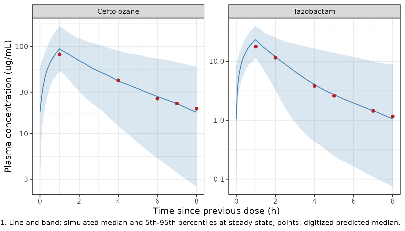
chk1 <- fig1 |>
  dplyr::inner_join(
    pct |> dplyr::filter(cohort == "ASPECT-NP") |> dplyr::select(drug, tad, Cc_q50),
    by = c("drug", "tad")
  ) |>
  dplyr::mutate(pct_diff = 100 * (Cc_q50 - pred_median) / pred_median)
chk1 |>
  dplyr::mutate(dplyr::across(c(Cc_q50, pct_diff), ~ signif(.x, 3))) |>
  dplyr::rename("Drug" = drug, "Time since dose (h)" = tad,
                "Digitized median" = pred_median, "Simulated median" = Cc_q50,
                "Difference (%)" = pct_diff) |>
knitr::kable()| Drug | Time since dose (h) | Digitized median | Simulated median | Difference (%) |
|---|---|---|---|---|
| Ceftolozane | 1 | 81.40 | 94.20 | 15.700 |
| Ceftolozane | 4 | 40.90 | 40.20 | -1.660 |
| Ceftolozane | 6 | 25.20 | 26.70 | 5.940 |
| Ceftolozane | 7 | 22.20 | 22.00 | -0.759 |
| Ceftolozane | 8 | 19.30 | 17.60 | -8.650 |
| Tazobactam | 1 | 17.80 | 23.40 | 31.500 |
| Tazobactam | 2 | 11.50 | 12.10 | 5.120 |
| Tazobactam | 4 | 3.82 | 4.05 | 6.150 |
| Tazobactam | 5 | 2.61 | 2.73 | 4.770 |
| Tazobactam | 7 | 1.44 | 1.45 | 0.487 |
| Tazobactam | 8 | 1.16 | 1.05 | -9.260 |
# Centre and robust envelope only: the VPC is binned over time since dose and
# the cohort covariates are reconstructed from Table 1 summaries. A wrong
# clearance, volume or dose shifts every point by tens of percent.
stopifnot(
  nrow(chk1) == nrow(fig1),
  abs(median(chk1$pct_diff)) < 15,
  quantile(abs(chk1$pct_diff), 0.9) < 30
)
Figure 4: ELF VPC in healthy participants and pneumonia patients
pct |>
  dplyr::filter(cohort != "ASPECT-NP", tad >= 0.5) |>
  ggplot(aes(tad)) +
  geom_ribbon(aes(ymin = Celf_q05, ymax = Celf_q95), fill = "steelblue", alpha = 0.2) +
  geom_line(aes(y = Celf_q50), colour = "steelblue") +
  geom_point(data = fig4, aes(y = pred_median), colour = "firebrick") +
  facet_wrap(cohort ~ drug, scales = "free_y") +
  scale_y_log10() +
  labs(x = "Time since previous dose (h)", y = "ELF concentration (ug/mL)",
       caption = paste("Replicates Figure 4 of Zhang 2021. Line and band: simulated",
                       "median and 5th-95th percentiles; points: digitized predicted",
                       "median.")) +
  theme_bw()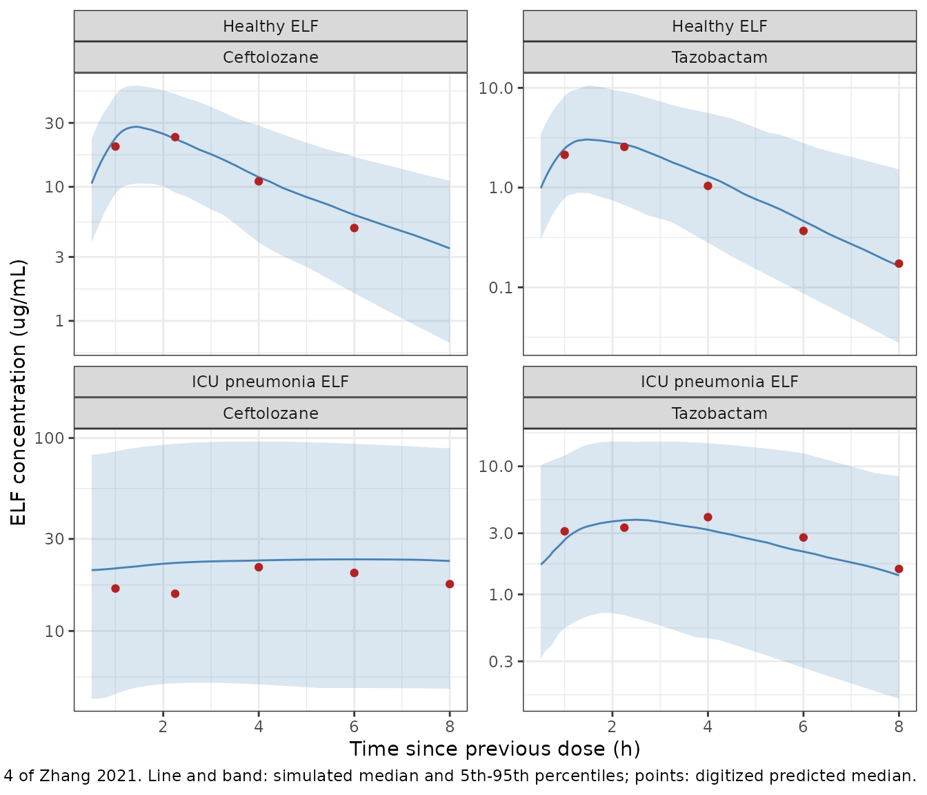
chk4 <- fig4 |>
  dplyr::inner_join(pct |> dplyr::select(drug, cohort, tad, Celf_q50),
                    by = c("drug", "cohort", "tad")) |>
  dplyr::mutate(pct_diff = 100 * (Celf_q50 - pred_median) / pred_median)
chk4 |>
  dplyr::mutate(dplyr::across(c(Celf_q50, pct_diff), ~ signif(.x, 3))) |>
  dplyr::rename("Drug" = drug, "Cohort" = cohort, "Time since dose (h)" = tad,
                "Digitized median" = pred_median, "Simulated median" = Celf_q50,
                "Difference (%)" = pct_diff) |>
knitr::kable()| Drug | Cohort | Time since dose (h) | Digitized median | Simulated median | Difference (%) |
|---|---|---|---|---|---|
| Ceftolozane | Healthy ELF | 1.00 | 20.000 | 23.100 | 15.70 |
| Ceftolozane | Healthy ELF | 2.25 | 23.500 | 22.800 | -2.86 |
| Ceftolozane | Healthy ELF | 4.00 | 11.000 | 11.800 | 7.32 |
| Ceftolozane | Healthy ELF | 6.00 | 4.930 | 6.180 | 25.30 |
| Tazobactam | Healthy ELF | 1.00 | 2.130 | 2.460 | 15.60 |
| Tazobactam | Healthy ELF | 2.25 | 2.560 | 2.730 | 6.49 |
| Tazobactam | Healthy ELF | 4.00 | 1.040 | 1.300 | 24.70 |
| Tazobactam | Healthy ELF | 6.00 | 0.368 | 0.462 | 25.50 |
| Tazobactam | Healthy ELF | 8.00 | 0.173 | 0.164 | -5.46 |
| Ceftolozane | ICU pneumonia ELF | 1.00 | 16.600 | 21.100 | 27.20 |
| Ceftolozane | ICU pneumonia ELF | 2.25 | 15.600 | 22.500 | 44.40 |
| Ceftolozane | ICU pneumonia ELF | 4.00 | 21.400 | 23.200 | 8.44 |
| Ceftolozane | ICU pneumonia ELF | 6.00 | 20.000 | 23.500 | 17.50 |
| Ceftolozane | ICU pneumonia ELF | 8.00 | 17.500 | 23.100 | 31.70 |
| Tazobactam | ICU pneumonia ELF | 1.00 | 3.110 | 2.670 | -14.30 |
| Tazobactam | ICU pneumonia ELF | 2.25 | 3.320 | 3.790 | 14.30 |
| Tazobactam | ICU pneumonia ELF | 4.00 | 4.010 | 3.200 | -20.30 |
| Tazobactam | ICU pneumonia ELF | 6.00 | 2.780 | 2.160 | -22.40 |
| Tazobactam | ICU pneumonia ELF | 8.00 | 1.580 | 1.410 | -10.90 |
chk4_hv <- chk4 |> dplyr::filter(cohort == "Healthy ELF")
chk4_icu <- chk4 |> dplyr::filter(cohort == "ICU pneumonia ELF")
# The paper's Figure 4 predictions come from the joint plasma-ELF fit, whose
# plasma parameters are not published, and the ELF cohorts' covariates are
# assumed; so only the centre and a robust envelope are gated.
stopifnot(
  nrow(chk4) == nrow(fig4),
  abs(median(chk4_hv$pct_diff)) < 30,
  abs(median(chk4_icu$pct_diff)) < 30,
  quantile(abs(chk4$pct_diff), 0.9) < 50
)
PKNCA validation
Steady-state NCA over the last dosing interval of the ASPECT-NP cohort, for plasma and ELF of both analytes.
run_nca <- function(sim, dose_col, drug) {
  conc <- sim |>
    dplyr::filter(cohort == "ASPECT-NP") |>
    dplyr::select(id, time, Cc, Celf) |>
    tidyr::pivot_longer(c(Cc, Celf), names_to = "matrix", values_to = "conc") |>
    dplyr::filter(!is.na(conc)) |>
    dplyr::mutate(treatment = drug)
  conc_obj <- PKNCA::PKNCAconc(conc, conc ~ time | treatment + id / matrix)
  dose_df <- subjects |>
    dplyr::filter(cohort == "ASPECT-NP") |>
    tidyr::crossing(time = seq(0, 152, by = 8)) |>
    dplyr::transmute(id, time, amt = .data[[dose_col]], treatment = drug)
  dose_obj <- PKNCA::PKNCAdose(dose_df, amt ~ time | treatment + id)
  intervals <- data.frame(start = 152, end = 160, cmax = TRUE, tmax = TRUE,
                          cmin = TRUE, auclast = TRUE)
  PKNCA::pk.nca(PKNCA::PKNCAdata(conc_obj, dose_obj, intervals = intervals))
}
nca_cef <- run_nca(sim_cef, "dose_cef", "Ceftolozane")
nca_taz <- run_nca(sim_taz, "dose_taz", "Tazobactam")

nca_wide <- dplyr::bind_rows(as.data.frame(nca_cef), as.data.frame(nca_taz)) |>
  dplyr::select(treatment, id, matrix, PPTESTCD, PPORRES) |>
  tidyr::pivot_wider(names_from = PPTESTCD, values_from = PPORRES)

nca_wide |>
  dplyr::group_by(treatment, matrix) |>
  dplyr::summarise(
    dplyr::across(c(cmax, cmin, auclast), ~ signif(median(.x), 3)),
    .groups = "drop"
  ) |>
  dplyr::rename("Drug" = treatment, "Matrix" = matrix, "Median Cmax (ug/mL)" = cmax,
                "Median Cmin (ug/mL)" = cmin, "Median AUCtau (h*ug/mL)" = auclast) |>
knitr::kable()| Drug | Matrix | Median Cmax (ug/mL) | Median Cmin (ug/mL) | Median AUCtau (h*ug/mL) |
|---|---|---|---|---|
| Ceftolozane | Cc | 94.20 | 17.60 | 361.0 |
| Ceftolozane | Celf | 24.20 | 22.20 | 188.0 |
| Tazobactam | Cc | 23.40 | 1.05 | 55.2 |
| Tazobactam | Celf | 4.02 | 1.33 | 21.5 |
Identity checks at steady state
Both checks compare a PKNCA result against a closed form built from the same drawn per-subject parameters, so the difference is pure trapezoidal error and a tight bound is the correct gate.
- Plasma:
AUCtau = Dose / CL. - ELF:
AUCtau(ELF) / AUCtau(plasma) = K1E / KE0, which holds only if the ELF compartment is a non-depleting link with volume equal to Vc.
indiv <- dplyr::bind_rows(
  sim_cef |> dplyr::mutate(treatment = "Ceftolozane", dose = dose_cef),
  sim_taz |> dplyr::mutate(treatment = "Tazobactam", dose = dose_taz)
) |>
  dplyr::filter(cohort == "ASPECT-NP") |>
  dplyr::group_by(treatment, id) |>
  dplyr::summarise(cl = dplyr::first(cl), ratio_expected = dplyr::first(k_central_elf / ke0),
                   dose = dplyr::first(dose), .groups = "drop")

ident <- nca_wide |>
  dplyr::select(treatment, id, matrix, auclast) |>
  tidyr::pivot_wider(names_from = matrix, values_from = auclast) |>
  dplyr::inner_join(indiv, by = c("treatment", "id")) |>
  dplyr::mutate(
    pct_auc = 100 * (Cc - dose / cl) / (dose / cl),
    pct_ratio = 100 * (Celf / Cc - ratio_expected) / ratio_expected
  )
ident |>
  dplyr::group_by(treatment) |>
  dplyr::summarise(
    median_auc = median(pct_auc), q90_auc = quantile(abs(pct_auc), 0.9),
    median_ratio = median(pct_ratio), q90_ratio = quantile(abs(pct_ratio), 0.9),
    .groups = "drop"
  ) |>
  dplyr::mutate(dplyr::across(-treatment, ~ signif(.x, 3))) |>
  dplyr::rename("Drug" = treatment,
                "AUCtau vs Dose/CL, median (%)" = median_auc,
                "AUCtau vs Dose/CL, 90th pct abs (%)" = q90_auc,
                "ELF/plasma vs K1E/KE0, median (%)" = median_ratio,
                "ELF/plasma vs K1E/KE0, 90th pct abs (%)" = q90_ratio) |>
knitr::kable()| Drug | AUCtau vs Dose/CL, median (%) | AUCtau vs Dose/CL, 90th pct abs (%) | ELF/plasma vs K1E/KE0, median (%) | ELF/plasma vs K1E/KE0, 90th pct abs (%) |
|---|---|---|---|---|
| Ceftolozane | 0.00779 | 0.0208 | -0.0447 | 0.0601 |
| Tazobactam | 0.01200 | 0.0263 | -0.0572 | 0.0733 |
ELF penetration
The paper reports no NCA table of its own. Its Discussion notes that
the link model assumption “seemed to work reasonably with previously
observed ceftolozane and tazobactam lung penetration ratios of 50% and
62%, respectively” (from the ICU ELF study). The model’s typical
steady-state ELF-to-plasma AUC ratio is K1E / KE0 from
Table 3:
tibble::tibble(
  drug = c("Ceftolozane", "Tazobactam"),
  model = c(0.808 / 1.56, 0.262 / 0.691),
  cited_observed = c(0.50, 0.62)
) |>
  dplyr::mutate(model = signif(model, 3)) |>
  dplyr::rename("Drug" = drug, "Model K1E/KE0" = model,
                "Observed ratio cited in the Discussion" = cited_observed) |>
knitr::kable()| Drug | Model K1E/KE0 | Observed ratio cited in the Discussion |
|---|---|---|
| Ceftolozane | 0.518 | 0.50 |
| Tazobactam | 0.379 | 0.62 |
Ceftolozane agrees (0.52 vs 0.50). For tazobactam the Table 3 point estimates imply 0.38, below the cited 0.62. Table 3 footnote c reports K1E and KE0 as highly correlated (r^2 >= 0.810), the pneumonia effect has a 44% RSE, and the cited ratio comes from a separate non-compartmental analysis, so the difference is recorded here rather than adjusted; the packaged model carries the printed estimates.
Assumptions and deviations
- Plasma component of the ELF model. The ELF link parameters (Table 3) were estimated jointly with a plasma model fitted to the data without the phase 3 studies, whose parameters are not reported (“data not shown”). The paper states that “The final ceftolozane and tazobactam ELF disposition models were the plasma models described above with a hypothetical ELF compartment linked to the plasma compartment”, so each packaged model combines the Table 2 plasma model with the Table 3 link.
- ELF residual error. The Table 3 residual error is applied to the ELF output and the Table 2 residual error to plasma. The paper does not say whether the joint fit used one residual model for both matrices.
- Pneumonia factor precision. Table 3 prints the ceftolozane factor as 0.034; the equations beneath it give 0.0339, which is used.
-
Typesetting in the source. The tazobactam Vp
equation drops the multiplication sign before
2.06^Pneumonia, and Table 2 footnote d labels the plasma %CV range as “(1-200 ug/mL)” although the printed “100%” end is reached at 0.1 ug/mL (at 1 ug/mL the formula gives 18.6%). Neither affects the model. -
Pneumonia column. The paper’s pneumonia stratum
pools ASPECT-NP HABP/VABP patients and critically ill patients with
confirmed or suspected pneumonia without separating hospital-acquired
from ventilator-associated pneumonia, so the unqualified
DIS_PNEUMONIAindicator carries it. -
Other infection.
DIS_OTHER_INFECTis the paper’s residual “other infection” type (critically ill patients with augmented renal clearance, CrCL >= 180 mL/min, in study MK-7625A-007). It is not an augmented-renal- clearance flag: ASPECT-NP patients with high CrCL are pneumonia patients in this model. - ESRD. The ESRD factors multiply the continuous CrCL term (the paper’s “in addition to the decrease associated with reduced CrCL”). They were estimated from 6 hemodialysis patients sampled after dialysis; the model does not describe clearance during dialysis.
- Covariates held at baseline, as in the paper.
- Virtual cohorts. Covariate distributions are reconstructed from Table 1 means and ranges; the ELF-study subgroup demographics are not printed and are assumed as described under Virtual cohorts. The digitized figure medians are approximate readings of raster images.