Pemetrexed + osimertinib sequence-dependent synergy QSP model (Hu 2026)
Source:vignettes/articles/Hu_2026_pemetrexed_osimertinib_mouse_qsp.Rmd
Hu_2026_pemetrexed_osimertinib_mouse_qsp.RmdModel and source
ui <- rxode2::rxode(readModelDb("Hu_2026_pemetrexed_osimertinib_mouse_qsp"))
#> ℹ parameter labels from comments will be replaced by 'label()'- Citation: Hu K, Lin Y, Ji H, Yuan T, Xia Y, Yang J. A Mechanistic Pharmacokinetic/Pharmacodynamic Model for Sequence-Dependent Synergy in Pemetrexed-Osimertinib Combinations Against Non-Small Cell Lung Cancer (NSCLC): Translational Insights. Pharmaceutics. 2026;18(4):408. doi:10.3390/pharmaceutics18040408.
- Article: https://doi.org/10.3390/pharmaceutics18040408
- Supplement (Tables S17-S21, the complete ODE system, parameter table, initial values and reaction scheme): https://www.mdpi.com/article/10.3390/pharmaceutics18040408/s1
Hu 2026 asks why the pemetrexed (PEM) + osimertinib (OSI) combination is schedule dependent: giving PEM first and OSI 48 h later is markedly more effective than giving both concurrently, even though the total dose of each agent is the same. The paper first rules out a pharmacokinetic explanation – no drug-drug interaction was detectable at the level of cellular uptake, systemic plasma exposure or intratumoral distribution – and then builds a mechanistic quantitative-systems-pharmacology (QSP) PK-PD model in which the schedule dependence emerges from the model structure alone. There is no schedule-specific interaction parameter: one parameter set reproduces every arm.
The mechanism the model encodes is a relay. PEM depletes the
folate-metabolizing enzyme pool and hence folate, which pushes
proliferating tumour cells into a damaged, non-proliferating state.
Those damaged cells drive a compensatory rebound of EGFR synthesis – a
pro-survival signal. OSI then does two things at once: it depletes EGFR
signal (suppressing that rebound) and, through the pro-apoptotic protein
Bim (for which the model uses 1 - EGFR as a surrogate),
accelerates the transit of damaged cells to death. But OSI also causes
G1 arrest, which blocks the proliferating-to-damaged transition
PEM depends on. Give OSI too early and the antagonism dominates; give it
after the damaged-cell pool has built up and the synergy dominates.
QSP. Preclinical (mouse, female BALB/c nude with subcutaneous HCC827 EGFR-mutant NSCLC xenograft). Mechanistic QSP-PK-PD model for the sequence-dependent synergy between pemetrexed (PEM) and the third-generation EGFR-TKI osimertinib (OSI). Five coupled modules: two-compartment PEM PK (intraperitoneal), two-compartment OSI PK (oral), a folate module in which PEM accelerates degradation of the folate-metabolizing enzyme pool and thereby depletes folate, an EGFR module in which OSI depletes EGFR signal while damaged tumour cells drive a compensatory rebound of EGFR synthesis, and a Simeoni-type tumour-growth-inhibition module (one proliferating pool plus a three-state damaged-cell transit chain). Folate depletion accelerates the proliferating-to-damaged transition; EGFR suppression both slows proliferation and (via the Bim surrogate 1 - EGFR) accelerates apoptosis of damaged cells, while EGFR-driven G1 arrest antagonises the proliferating-to-damaged transition. Sequence dependence emerges from the model structure and dosing schedule alone – no schedule-specific interaction parameter is fitted. An unperturbed (drug-free) twin tumour chain is carried alongside so real-time TGI% can be computed. Parameter values from Hu 2026 supplementary Tables S17-S21.
Population
| Field | Value |
|---|---|
| species | mouse (female BALB/c nude with subcutaneous HCC827 EGFR-mutant NSCLC xenograft); PK parameters from PC9-bearing male/female BALB/c nude mice |
| n_subjects | 25 |
| n_studies | 1 |
| age_range | 7 weeks at inoculation |
| weight_range | approximately 20 g |
| sex_female_pct | 100 |
| race_ethnicity | NA |
| disease_state | subcutaneous HCC827 human EGFR-exon-19-deletion NSCLC xenograft (1e7 cells in 50% high-concentration Matrigel, right flank); randomised at a tumour volume of approximately 200 mm3 |
| dose_range | pemetrexed 35 mg/kg intraperitoneally three times daily 4 h apart (105 mg/kg/day) on days 0-1 of each 7-day cycle; osimertinib 1 mg/kg orally once daily on days 0-2 (concurrent) or days 2-4 (48 h sequential) of each cycle; three cycles |
| regions | preclinical (China Pharmaceutical University, Nanjing, China; animal ethics approval YSL-202504062) |
| notes | Five arms of n = 5 (control, PEM, OSI, PEM + OSI, PEM -> OSI); tumour volume V = (pi/6) * a * b^2 measured by caliper every 3 days to day 18 (Hu 2026 Figure 6B, replotted from the authors’ earlier report, Hu 2025, Pharmaceutics 17:1044, doi:10.3390/pharmaceutics17081044). The PK sub-models were fitted separately in WinNonlin to pooled mean plasma profiles from PC9-bearing BALB/c nude mice dosed pemetrexed 100 mg/kg i.p. and osimertinib 5 mg/kg p.o. (Hu 2026 Figures 5D and S4A,B). Between-subject variability is the 30% CV log-normal spread applied to every PD and tumour-growth parameter in the Monte Carlo analysis of Hu 2026 Supplementary Method S1.7. |
The efficacy experiment (Hu 2026 Figure 6, replotted from the authors’ earlier pharmacodynamic study) used female BALB/c nude mice bearing subcutaneous HCC827 xenografts, randomised at a tumour volume of about 200 mm^3 into five arms of five animals: vehicle control, PEM alone, OSI alone, concurrent PEM + OSI, and sequential PEM to OSI with a 48 h interval. Tumour volume was measured by caliper every three days to day 18. The PK sub-models were fitted separately, in WinNonlin, to pooled mean plasma profiles from PC9-bearing BALB/c nude mice (Hu 2026 Figures 5D and S4A,B).
Source trace
Every ini() entry in
inst/modeldb/specificDrugs/Hu_2026_pemetrexed_osimertinib_mouse_qsp.R
carries an in-file comment naming its origin. The table below collects
them. Unless stated otherwise the source is Hu 2026 supplementary Table
S19, whose “Source” column also determines which parameters are wrapped
in fixed(): rows sourced from Assumed Value or
Literature are fixed, rows sourced from Curve Fitting,
PK Analysis, in vitro data or IVIVE are left
free.
| Equation / parameter | Value | Source location |
|---|---|---|
d/dt(depot), d/dt(central),
d/dt(peripheral1)
|
n/a | Equations (1)-(3); Table S17 rows 10-12 |
d/dt(depot_osimertinib),
d/dt(central_osimertinib),
d/dt(peripheral1_osimertinib)
|
n/a | Equations (4)-(6); Table S17 rows 15-17 |
d/dt(enzyme_folate), d/dt(folate)
|
n/a | Equations (7)-(8); Table S17 rows 13-14 |
d/dt(egfr_signal) |
n/a | Equation (9); Table S17 row 18 |
d/dt(cycling_cells) …
d/dt(damaged_cells3), d/dt(total_death)
|
n/a | Equations (10)-(13), (17); Table S17 rows 1-4, 9 |
d/dt(*_unperturbed) |
n/a | Supplementary Equations (S1)-(S4); Table S17 rows 5-8 |
x_total, damaged_frac,
x1_fraction, tgi
|
n/a | Equations (14)-(16); Table S18 rows 1-6 |
lka (ka_pem) |
102.3379 1/day | Table S19, PK Analysis |
lkel (kel_pem) |
56.6998 1/day | Table S19, PK Analysis |
lk12 (k12_pem) |
2.3398 1/day | Table S19, PK Analysis |
lk21 (k21_pem) |
2.8223 1/day | Table S19, PK Analysis |
lvc (PEM_V1) |
0.39125 L/kg | Table S19, PK Analysis |
lvp (PEM_V2) |
0.32436 L/kg | Table S19, PK Analysis |
lka_osimertinib |
24.6514 1/day | Table S19, PK Analysis |
lkel_osimertinib |
10.6071 1/day | Table S19, PK Analysis |
lk12_osimertinib |
11.005 1/day | Table S19, PK Analysis |
lk21_osimertinib |
5.4194 1/day | Table S19, PK Analysis |
lvc_osimertinib (OSI_V1/F) |
7.1758 L/kg | Table S19, PK Analysis |
lvp_osimertinib (OSI_V2/F) |
14.5716 L/kg | Table S19, PK Analysis |
lkout_enzyme (kout_Enzyme) |
1 1/day, fixed | Table S19, Assumed Value |
lkout_folate |
3 1/day, fixed | Table S19, Assumed Value |
lgamma_enzyme (gamma_Enzyme) |
2.0129 | Table S19, IVIVE |
lemax_enzyme (Emax_pem) |
5.56 | Table S19, IVIVE |
lec50_enzyme (EC50_pem,plasma) |
0.47315 mg/L | Table S19 / Supplementary Method S1.6, IVIVE from EC50 = 300 nM in medium |
lkout_egfr_signal (kout_EGFR) |
1.5 1/day | Table S19, IVIVE from Figure 7E,F |
lkfeedback_egfr_signal |
0.2 | Table S19, Curve Fitting |
lgamma_feedback_egfr_signal |
1.45 | Table S19, Curve Fitting |
limax_osimertinib (Imax_osi) |
22.872, fixed | Table S19, Literature (doi:10.1158/1535-7163.MCT-16-0142) |
lec50_osimertinib (EC50_osi,plasma) |
48.866 ug/L | Table S19, IVIVE from EC50 = 14.49 nM in medium (Figure 7G,H) |
lgamma_osimertinib (gamma_osi) |
2, fixed | Table S19, Assumed Value |
ltumorExpGrowth (Lambda_0) |
0.1032 1/day | Table S19, Curve Fitting (Figure 8E) |
ltumorLinGrowth (Lambda_1) |
51.08 mm3/day | Table S19, Curve Fitting (Figure 8E) |
ldamageRate (k1) |
0.016 1/day | Table S19, Curve Fitting |
ldamageTransit (k2) |
0.0045 1/day | Table S19, Curve Fitting |
lemax_folate (Emax_folate) |
49.5 | Table S19, IVIVE |
lec50_folate (EC50_folate) |
0.5, fixed | Table S19, Assumed Value |
lkbim (k_bim) |
211, fixed | Table S19, Literature (doi:10.1158/1535-7163.MCT-16-0142) |
lgamma_bim (gamma_bim) |
0.595 | Table S19, IVIVE from Figure 7L |
lgamma_g1_egfr_signal (gamma_G1) |
8, fixed | Table S19, Assumed Value |
lgamma_prolif_egfr_signal
(gamma_EGFR) |
3.998 | Table S19, IVIVE from Figure 7A,B |
psi |
20, fixed | Table S19, Literature (Simeoni 2004) |
tumor_vol0 |
200 mm3, fixed | Table S20, initial value of X1 |
| eta variances (all 21) | 0.0861777 = ln(1 + 0.30^2), fixed | Supplementary Method S1.7, Equations (S10)-(S12): 30% CV log-normal |
propSd_tumor_vol |
0, fixed | Not reported: Hu 2026 calibrates to mean tumour volumes and simulates only |
| BIM-deletion scenario |
k_bim 21.1, gamma_bim x 5, prevalence
11.5% |
Section 3.6 and Supplementary Method S1.7 |
| Dosing schedule | PEM 35 mg/kg i.p. t.i.d. 4 h apart on days 0-1; OSI 1 mg/kg p.o. on days 0-2 (concurrent) or 2-4 (sequential); 7-day cycle x 3 | Figure 6A and Section 2.2 |
Dosing schedule and event tables
Figure 6A defines a 7-day treatment cycle, repeated three times, with tumour volume followed to day 18. Pemetrexed is given intraperitoneally at 35 mg/kg three times daily 4 h apart (105 mg/kg/day) on days 0 and 1 of each cycle; osimertinib is given orally at 1 mg/kg once daily on days 0-2 in the concurrent arm and on days 2-4 in the 48 h sequential arm. Both combination arms therefore receive the same total dose of each drug – only the ordering differs.
cycle_start <- c(0, 7, 14)              # three 7-day cycles (Figure 6A)
pem_hours   <- c(0, 4, 8) / 24          # t.i.d., 4 h apart (Section 2.2)
pem_days    <- c(0, 1)                  # PEM on days 0 and 1 of each cycle
pem_times   <- sort(as.vector(outer(pem_hours,
                                    as.vector(outer(cycle_start, pem_days, "+")), "+")))
osi_concurrent <- sort(as.vector(outer(cycle_start, c(0, 1, 2), "+")))
osi_sequential <- sort(as.vector(outer(cycle_start, c(2, 3, 4), "+")))

pem_dose <- 35   # mg/kg per administration
osi_dose <- 1    # mg/kg per administration

# Observation rows carry no `cmt`, so rxode2 records every state and every
# algebraic observable at each time. Dose rows name the ODE STATE they enter.
make_events <- function(pem = NULL, osi = NULL, obs = seq(0, 18, by = 0.01), n = 1L) {
  ev <- rxode2::et(obs)
  if (!is.null(pem)) ev <- rxode2::et(ev, amt = pem_dose, cmt = "depot", time = pem)
  if (!is.null(osi)) ev <- rxode2::et(ev, amt = osi_dose, cmt = "depot_osimertinib", time = osi)
  if (n > 1L) ev <- rxode2::et(ev, id = seq_len(n))
  ev
}

arm_events <- list(
  "Control"    = make_events(),
  "PEM"        = make_events(pem = pem_times),
  "OSI"        = make_events(osi = osi_concurrent),
  "PEM + OSI"  = make_events(pem = pem_times, osi = osi_concurrent),
  "PEM -> OSI" = make_events(pem = pem_times, osi = osi_sequential)
)
Typical-value simulation of the five arms
Hu 2026 Figures 6B and 8 are typical-value predictions, so the random
effects are zeroed. rxSolve() is called once per arm (a
single call per arm is required: solving an rxUi is
quadratic in the number of subjects).
tv <- rxode2::zeroRe(ui)

solve_arm <- function(ev, name) {
  out <- as.data.frame(rxode2::rxSolve(tv, ev, atol = 1e-9, rtol = 1e-9))
  if (is.null(out$id)) out$id <- 1L      # rxSolve omits `id` for one subject
  out$arm <- name
  out
}
sim_arms <- dplyr::bind_rows(Map(solve_arm, arm_events, names(arm_events)))
#> ℹ omega/sigma items treated as zero: 'etalgamma_enzyme', 'etalemax_enzyme', 'etalec50_enzyme', 'etalkout_enzyme', 'etalkout_folate', 'etalkout_egfr_signal', 'etalkfeedback_egfr_signal', 'etalgamma_feedback_egfr_signal', 'etalimax_osimertinib', 'etalec50_osimertinib', 'etalgamma_osimertinib', 'etaltumorExpGrowth', 'etaltumorLinGrowth', 'etaldamageRate', 'etaldamageTransit', 'etalemax_folate', 'etalec50_folate', 'etalkbim', 'etalgamma_bim', 'etalgamma_g1_egfr_signal', 'etalgamma_prolif_egfr_signal'
#> ℹ omega/sigma items treated as zero: 'etalgamma_enzyme', 'etalemax_enzyme', 'etalec50_enzyme', 'etalkout_enzyme', 'etalkout_folate', 'etalkout_egfr_signal', 'etalkfeedback_egfr_signal', 'etalgamma_feedback_egfr_signal', 'etalimax_osimertinib', 'etalec50_osimertinib', 'etalgamma_osimertinib', 'etaltumorExpGrowth', 'etaltumorLinGrowth', 'etaldamageRate', 'etaldamageTransit', 'etalemax_folate', 'etalec50_folate', 'etalkbim', 'etalgamma_bim', 'etalgamma_g1_egfr_signal', 'etalgamma_prolif_egfr_signal'
#> ℹ omega/sigma items treated as zero: 'etalgamma_enzyme', 'etalemax_enzyme', 'etalec50_enzyme', 'etalkout_enzyme', 'etalkout_folate', 'etalkout_egfr_signal', 'etalkfeedback_egfr_signal', 'etalgamma_feedback_egfr_signal', 'etalimax_osimertinib', 'etalec50_osimertinib', 'etalgamma_osimertinib', 'etaltumorExpGrowth', 'etaltumorLinGrowth', 'etaldamageRate', 'etaldamageTransit', 'etalemax_folate', 'etalec50_folate', 'etalkbim', 'etalgamma_bim', 'etalgamma_g1_egfr_signal', 'etalgamma_prolif_egfr_signal'
#> ℹ omega/sigma items treated as zero: 'etalgamma_enzyme', 'etalemax_enzyme', 'etalec50_enzyme', 'etalkout_enzyme', 'etalkout_folate', 'etalkout_egfr_signal', 'etalkfeedback_egfr_signal', 'etalgamma_feedback_egfr_signal', 'etalimax_osimertinib', 'etalec50_osimertinib', 'etalgamma_osimertinib', 'etaltumorExpGrowth', 'etaltumorLinGrowth', 'etaldamageRate', 'etaldamageTransit', 'etalemax_folate', 'etalec50_folate', 'etalkbim', 'etalgamma_bim', 'etalgamma_g1_egfr_signal', 'etalgamma_prolif_egfr_signal'
#> ℹ omega/sigma items treated as zero: 'etalgamma_enzyme', 'etalemax_enzyme', 'etalec50_enzyme', 'etalkout_enzyme', 'etalkout_folate', 'etalkout_egfr_signal', 'etalkfeedback_egfr_signal', 'etalgamma_feedback_egfr_signal', 'etalimax_osimertinib', 'etalec50_osimertinib', 'etalgamma_osimertinib', 'etaltumorExpGrowth', 'etaltumorLinGrowth', 'etaldamageRate', 'etaldamageTransit', 'etalemax_folate', 'etalec50_folate', 'etalkbim', 'etalgamma_bim', 'etalgamma_g1_egfr_signal', 'etalgamma_prolif_egfr_signal'
sim_arms$arm <- factor(sim_arms$arm, levels = names(arm_events))
Structural checks
Before comparing to any published figure, three closed-form properties of the system are checked. They depend only on the printed parameter values, so they verify the ODE transcription independently of any simulated output.
# 1. Baseline homeostasis: with no drug the three normalised pools sit at 1.
ctl <- dplyr::filter(sim_arms, arm == "Control")
baseline_dev <- max(abs(ctl$folate - 1), abs(ctl$enzyme_folate - 1))

# 2. lambda0: switching off the damage chain leaves a pure Simeoni growth
#    curve whose early log-slope is exactly Lambda_0.
growth_only <- as.data.frame(rxode2::rxSolve(
  rxode2::ini(tv, ldamageRate = log(1e-10)),
  rxode2::et(seq(0, 3, by = 0.01)), atol = 1e-10, rtol = 1e-10))
#> ℹ change initial estimate of `ldamageRate` to `-23.0258509299405`
#> ℹ omega/sigma items treated as zero: 'etalgamma_enzyme', 'etalemax_enzyme', 'etalec50_enzyme', 'etalkout_enzyme', 'etalkout_folate', 'etalkout_egfr_signal', 'etalkfeedback_egfr_signal', 'etalgamma_feedback_egfr_signal', 'etalimax_osimertinib', 'etalec50_osimertinib', 'etalgamma_osimertinib', 'etaltumorExpGrowth', 'etaltumorLinGrowth', 'etaldamageRate', 'etaldamageTransit', 'etalemax_folate', 'etalec50_folate', 'etalkbim', 'etalgamma_bim', 'etalgamma_g1_egfr_signal', 'etalgamma_prolif_egfr_signal'
lam0_hat <- unname(coef(lm(
  log(x_total_unperturbed) ~ time,
  data = growth_only[growth_only$time > 0, ]))[2])

# 3. lambda1: the late phase of the unperturbed tumour is linear at Lambda_1.
long_ctl <- as.data.frame(rxode2::rxSolve(
  tv, rxode2::et(seq(0, 60, by = 0.05)), atol = 1e-10, rtol = 1e-10))
#> ℹ omega/sigma items treated as zero: 'etalgamma_enzyme', 'etalemax_enzyme', 'etalec50_enzyme', 'etalkout_enzyme', 'etalkout_folate', 'etalkout_egfr_signal', 'etalkfeedback_egfr_signal', 'etalgamma_feedback_egfr_signal', 'etalimax_osimertinib', 'etalec50_osimertinib', 'etalgamma_osimertinib', 'etaltumorExpGrowth', 'etaltumorLinGrowth', 'etaldamageRate', 'etaldamageTransit', 'etalemax_folate', 'etalec50_folate', 'etalkbim', 'etalgamma_bim', 'etalgamma_g1_egfr_signal', 'etalgamma_prolif_egfr_signal'
lam1_hat <- unname(coef(lm(
  x_total_unperturbed ~ time,
  data = long_ctl[long_ctl$time >= 40, ]))[2])

# 4. The untreated control tracks its own drug-free twin. It is not identical:
#    the twin chain omits the EGFR terms entirely, while in the control arm
#    damaged-cell feedback lifts EGFR a little above baseline, which slightly
#    accelerates proliferation. The published model has this property; the gap
#    is a few percent.
ctl_tgi <- max(abs(ctl$tgi))

structural <- tibble::tibble(
  Check = c("max |folate - 1| and |enzyme - 1|, untreated (target 0)",
            "lambda0 recovered from the damage-free growth curve (Table S19: 0.1032 1/day)",
            "lambda1 recovered from the late linear phase (Table S19: 51.08 mm3/day)",
            "max |TGI| in the untreated control (drug-free twin reference)",
            "EGFR recovery half-time ln(2)/kout_EGFR (Figure 7E,F: kout_EGFR = 1.5 1/day)"),
  Value = c(signif(baseline_dev, 3), signif(lam0_hat, 6), signif(lam1_hat, 6),
            signif(ctl_tgi, 3), signif(log(2) / 1.5 * 24, 4)),
  Unit  = c("", "1/day", "mm3/day", "fraction", "h")
)
knitr::kable(structural, caption = "Closed-form structural checks.")| Check | Value | Unit |
|---|---|---|
| max |folate - 1| and |enzyme - 1|, untreated (target 0) | 0.0000 | |
| lambda0 recovered from the damage-free growth curve (Table S19: 0.1032 1/day) | 0.1032 | 1/day |
| lambda1 recovered from the late linear phase (Table S19: 51.08 mm3/day) | 51.0638 | mm3/day |
| max |TGI| in the untreated control (drug-free twin reference) | 0.0226 | fraction |
| EGFR recovery half-time ln(2)/kout_EGFR (Figure 7E,F: kout_EGFR = 1.5 1/day) | 11.0900 | h |
Replicating Figure 6B and Figure 8
ggplot(sim_arms, aes(time, tumor_vol, colour = arm)) +
  geom_line(linewidth = 0.8) +
  scale_x_continuous(breaks = seq(0, 18, by = 3)) +
  labs(x = "Time (day)", y = expression("Tumour volume ("*mm^3*")"),
       colour = NULL,
       title = "Tumour volume under each combination strategy",
       caption = "Replicates Figure 6B and Figure 8A-E of Hu 2026.") +
  theme_bw()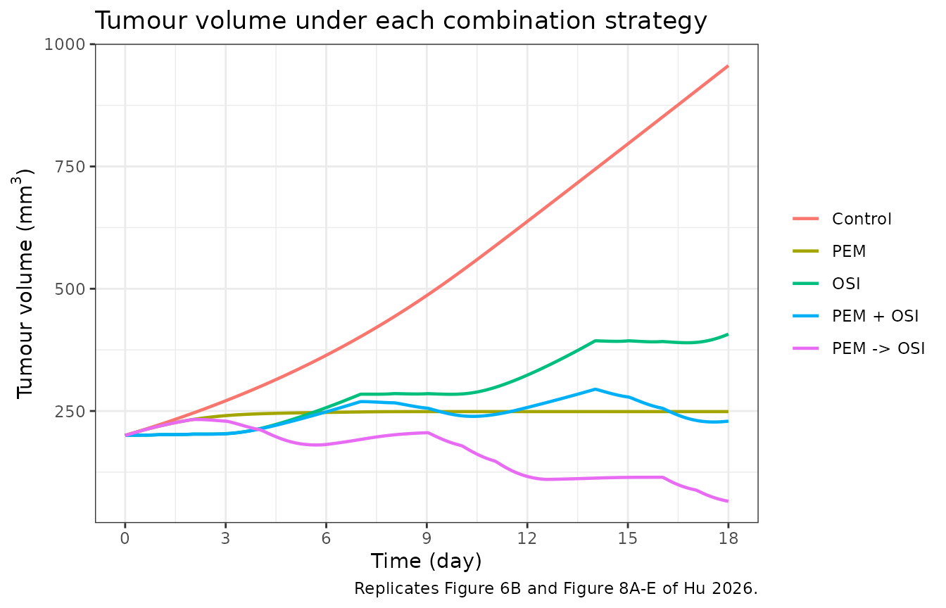
Replicates Figure 6B / Figure 8A-E of Hu 2026: typical-value tumour volume by arm.
At the day-18 endpoint Hu 2026 reports observed mean tumour volumes in the PEM + OSI and PEM to OSI groups equal to 64.5% and 22.3% of the OSI monotherapy group (Section 3.2). The paper’s own acceptance criterion for the model is that every observation lies within a two-fold range of the corresponding prediction (Figure 8F), so that is what is asserted here.
d18 <- sim_arms |>
  group_by(arm) |>
  slice_min(abs(time - 18), n = 1, with_ties = FALSE) |>
  ungroup() |>
  select(arm, tumor_vol)

osi_ref <- d18$tumor_vol[d18$arm == "OSI"]
endpoint <- d18 |>
  mutate(`Predicted, mm3`  = round(tumor_vol, 1),
         `Predicted, % OSI` = round(100 * tumor_vol / osi_ref, 1),
         `Observed, % OSI`  = c(NA, NA, 100, 64.5, 22.3)) |>
  mutate(`Predicted / observed` = round(`Predicted, % OSI` / `Observed, % OSI`, 3)) |>
  select(-tumor_vol) |>
  rename(Arm = arm)
knitr::kable(endpoint, caption = paste(
  "Day-18 tumour volume. Observed percentages are Hu 2026 Section 3.2;",
"the paper's stated acceptance criterion is agreement within two-fold."))| Arm | Predicted, mm3 | Predicted, % OSI | Observed, % OSI | Predicted / observed |
|---|---|---|---|---|
| Control | 956.3 | 234.9 | NA | NA |
| PEM | 248.8 | 61.1 | NA | NA |
| OSI | 407.2 | 100.0 | 100.0 | 1.000 |
| PEM + OSI | 229.3 | 56.3 | 64.5 | 0.873 |
| PEM -> OSI | 65.4 | 16.1 | 22.3 | 0.722 |
ratio <- endpoint$`Predicted / observed`[endpoint$Arm %in% c("PEM + OSI", "PEM -> OSI")]
stopifnot(
  # Sequence dependence emerges from the model structure alone.
  d18$tumor_vol[d18$arm == "PEM -> OSI"] < d18$tumor_vol[d18$arm == "PEM + OSI"],
  d18$tumor_vol[d18$arm == "PEM + OSI"]  < d18$tumor_vol[d18$arm == "OSI"],
  d18$tumor_vol[d18$arm == "OSI"]        < d18$tumor_vol[d18$arm == "Control"],
  # Hu 2026 Figure 8F: observations within two-fold of predictions.
  all(ratio > 0.5), all(ratio < 2)
)
Replicating Figure S4C-F: the simulated plasma profiles
Figure S4C plots simulated pemetrexed plasma concentration over the 18-day study on a 0-50 mg/L axis with peaks a little above 40 mg/L; Figure S4D plots osimertinib on a 0-80 ug/L axis with peaks just below 60 ug/L.
sim_arms |>
  filter(arm %in% c("PEM + OSI", "PEM -> OSI")) |>
  select(time, arm, PEM = Cc, OSI = Cc_osimertinib) |>
  pivot_longer(c(PEM, OSI), names_to = "Drug", values_to = "conc") |>
  ggplot(aes(time, conc, colour = Drug)) +
  geom_line(linewidth = 0.4) +
  facet_wrap(~arm, ncol = 1) +
  scale_x_continuous(breaks = seq(0, 18, by = 3)) +
  labs(x = "Time (day)", y = "Concentration (mg/L for PEM, ug/L for OSI)",
       title = "Simulated plasma concentration-time profiles",
       caption = "Replicates Figure S4E,F of Hu 2026.") +
  theme_bw()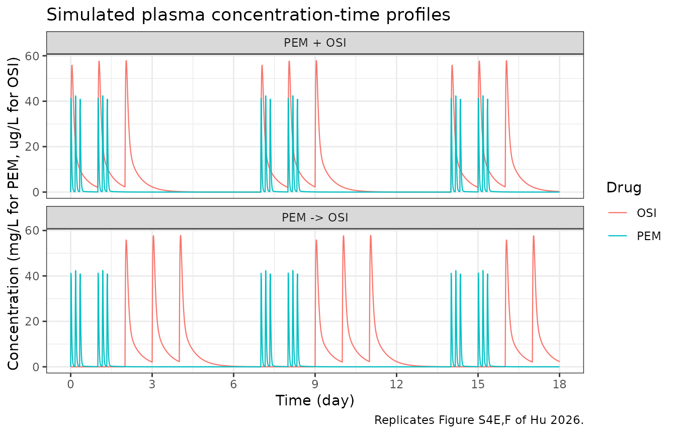
Replicates Figure S4E,F of Hu 2026: plasma profiles in the two combination arms.
peaks <- tibble::tibble(
  Drug        = c("Pemetrexed", "Osimertinib"),
  `Simulated peak` = c(round(max(sim_arms$Cc), 2), round(max(sim_arms$Cc_osimertinib), 2)),
  `Hu 2026 peak`   = c(42, 57),
  Unit        = c("mg/L", "ug/L"),
  Source      = c("Figure S4C", "Figure S4D")
)
knitr::kable(peaks, caption = "Simulated peak plasma concentrations versus Hu 2026 Figures S4C and S4D.")| Drug | Simulated peak | Hu 2026 peak | Unit | Source |
|---|---|---|---|---|
| Pemetrexed | 42.38 | 42 | mg/L | Figure S4C |
| Osimertinib | 57.86 | 57 | ug/L | Figure S4D |
PKNCA validation of the PK layer
Non-compartmental analysis of a single dose of each drug is compared
against closed-form values derived analytically from the printed
micro-constants of Table S19. This is an independent check that the ODE
system integrates to the exposure the published parameters imply:
AUC(0-inf) = dose / (kel * V1) and the terminal half-life
is ln(2) / beta, where beta is the smaller
root of the two-compartment characteristic equation.
# Both drugs are expressed in ug/L so a single PKNCA analysis covers them.
pk_grid <- sort(unique(c(seq(0, 0.2, by = 0.0005), seq(0.2, 8, by = 0.002))))

pk_pem <- as.data.frame(rxode2::rxSolve(
  tv, make_events(pem = 0, obs = pk_grid), atol = 1e-10, rtol = 1e-10)) |>
  transmute(id = 1L, time, conc = 1000 * Cc,
            treatment = "Pemetrexed 35 mg/kg i.p.")
#> ℹ omega/sigma items treated as zero: 'etalgamma_enzyme', 'etalemax_enzyme', 'etalec50_enzyme', 'etalkout_enzyme', 'etalkout_folate', 'etalkout_egfr_signal', 'etalkfeedback_egfr_signal', 'etalgamma_feedback_egfr_signal', 'etalimax_osimertinib', 'etalec50_osimertinib', 'etalgamma_osimertinib', 'etaltumorExpGrowth', 'etaltumorLinGrowth', 'etaldamageRate', 'etaldamageTransit', 'etalemax_folate', 'etalec50_folate', 'etalkbim', 'etalgamma_bim', 'etalgamma_g1_egfr_signal', 'etalgamma_prolif_egfr_signal'

pk_osi <- as.data.frame(rxode2::rxSolve(
  tv, make_events(osi = 0, obs = pk_grid), atol = 1e-10, rtol = 1e-10)) |>
  transmute(id = 1L, time, conc = Cc_osimertinib,
            treatment = "Osimertinib 1 mg/kg p.o.")
#> ℹ omega/sigma items treated as zero: 'etalgamma_enzyme', 'etalemax_enzyme', 'etalec50_enzyme', 'etalkout_enzyme', 'etalkout_folate', 'etalkout_egfr_signal', 'etalkfeedback_egfr_signal', 'etalgamma_feedback_egfr_signal', 'etalimax_osimertinib', 'etalec50_osimertinib', 'etalgamma_osimertinib', 'etaltumorExpGrowth', 'etaltumorLinGrowth', 'etaldamageRate', 'etaldamageTransit', 'etalemax_folate', 'etalec50_folate', 'etalkbim', 'etalgamma_bim', 'etalgamma_g1_egfr_signal', 'etalgamma_prolif_egfr_signal'

sim_nca <- bind_rows(pk_pem, pk_osi) |>
  filter(!is.na(conc)) |>
  # Per subject, keep conc >= 1e-6 * Cmax after the peak: below that the ODE integrator has no relative accuracy left.
  group_by(treatment, id) |>
  filter(time <= time[which.max(conc)] | conc >= 1e-6 * max(conc)) |>
  ungroup() |>
  select(id, time, conc, treatment)

# Guarantee a time-zero row per (id, treatment); pre-dose concentration is 0
# for both extravascular routes.
sim_nca <- bind_rows(
  sim_nca,
  sim_nca |> distinct(id, treatment) |> mutate(time = 0, conc = 0)
) |>
  distinct(id, treatment, time, .keep_all = TRUE) |>
  arrange(treatment, id, time)

dose_df <- bind_rows(
  tibble::tibble(id = 1L, time = 0, amt = pem_dose * 1e6,
                 treatment = "Pemetrexed 35 mg/kg i.p."),
  tibble::tibble(id = 1L, time = 0, amt = osi_dose * 1e6,
                 treatment = "Osimertinib 1 mg/kg p.o.")
)

conc_obj <- PKNCA::PKNCAconc(sim_nca, conc ~ time | treatment + id)
dose_obj <- PKNCA::PKNCAdose(dose_df, amt ~ time | treatment + id)

intervals <- data.frame(start = 0, end = Inf,
                        cmax = TRUE, tmax = TRUE,
                        aucinf.obs = TRUE, half.life = TRUE)

nca_res <- PKNCA::pk.nca(PKNCA::PKNCAdata(conc_obj, dose_obj, intervals = intervals))
# Closed-form reference values from the Table S19 micro-constants.
beta_terminal <- function(kel, k12, k21) {
  s <- kel + k12 + k21
  0.5 * (s - sqrt(s^2 - 4 * kel * k21))
}
pem_beta <- beta_terminal(56.6998, 2.3398, 2.8223)
osi_beta <- beta_terminal(10.6071, 11.005, 5.4194)

published <- tibble::tribble(
  ~treatment,                    ~cmax,  ~tmax,          ~aucinf.obs,                      ~half.life,
  "Pemetrexed 35 mg/kg i.p.",    42000,  18 / (24 * 60), 1e3 * pem_dose / (56.6998 * 0.39125), log(2) / pem_beta,
  "Osimertinib 1 mg/kg p.o.",    57,     1.1 / 24,       1e3 * osi_dose / (10.6071 * 7.1758),  log(2) / osi_beta
)

cmp <- nlmixr2lib::ncaComparisonTable(
  simulated = nca_res,
  reference = published,
  by        = "treatment",
  units     = c(cmax = "ug/L", aucinf.obs = "ug*day/L",
                tmax = "day", half.life = "day"),
  tolerance_pct = 20
)
knitr::kable(cmp, caption = paste(
  "Simulated NCA versus reference. AUC(0-inf) and half-life references are",
  "closed-form from the Table S19 micro-constants; Cmax and Tmax references",
"are read from Hu 2026 Figures S4A-D. * marks a >20% difference."))| NCA parameter | treatment | Reference | Simulated | % diff |
|---|---|---|---|---|
| Cmax (ug/L) | Pemetrexed 35 mg/kg i.p. | 42000 | 42300 | +0.6% |
| Cmax (ug/L) | Osimertinib 1 mg/kg p.o. | 57 | 56 | -1.7% |
| Tmax (day) | Pemetrexed 35 mg/kg i.p. | 0.0125 | 0.0125 | +0.0% |
| Tmax (day) | Osimertinib 1 mg/kg p.o. | 0.0458 | 0.046 | +0.4% |
| AUC0-∞ (obs) (ug*day/L) | Pemetrexed 35 mg/kg i.p. | 1580 | 1580 | -0.0% |
| AUC0-∞ (obs) (ug*day/L) | Osimertinib 1 mg/kg p.o. | 13.1 | 13.1 | -0.0% |
| t½ (day) | Pemetrexed 35 mg/kg i.p. | 0.256 | 0.255 | -0.3% |
| t½ (day) | Osimertinib 1 mg/kg p.o. | 0.298 | 0.297 | -0.3% |
get_nca <- function(res, trt, code) {
  d <- as.data.frame(res)
  d$PPORRES[d$treatment == trt & d$PPTESTCD == code][1]
}
auc_pem <- get_nca(nca_res, "Pemetrexed 35 mg/kg i.p.",  "aucinf.obs")
auc_osi <- get_nca(nca_res, "Osimertinib 1 mg/kg p.o.",  "aucinf.obs")
hl_pem  <- get_nca(nca_res, "Pemetrexed 35 mg/kg i.p.",  "half.life")
hl_osi  <- get_nca(nca_res, "Osimertinib 1 mg/kg p.o.",  "half.life")

stopifnot(
  # AUC(0-inf) must equal dose / CL to within numerical-integration error.
  abs(auc_pem / (1e3 * pem_dose / (56.6998 * 0.39125)) - 1) < 0.01,
  abs(auc_osi / (1e3 * osi_dose / (10.6071 * 7.1758))  - 1) < 0.01,
  # Terminal half-life must equal ln(2) / beta.
  abs(hl_pem / (log(2) / pem_beta) - 1) < 0.05,
  abs(hl_osi / (log(2) / osi_beta) - 1) < 0.05
)
Replicating Figure 10: the optimal sequential interval
Hu 2026 Section 3.5 simulates the sequential regimen at 24, 48, 72 and 96 h intervals and reports that “the final simulated tumour volume under the 48 h interval PEM to OSI schedule was less than half of that simulated with the 24 h interval, while extending the interval to 72 h or 96 h offered negligible additional benefits”.
interval_days <- c(1, 2, 3, 4)
interval_sim <- lapply(interval_days, function(k) {
  ev <- make_events(pem = pem_times,
                    osi = sort(as.vector(outer(cycle_start, k + c(0, 1, 2), "+"))))
  out <- as.data.frame(rxode2::rxSolve(tv, ev, atol = 1e-9, rtol = 1e-9))
  out$interval <- paste0(k * 24, " h")
  out
}) |> bind_rows()
#> ℹ omega/sigma items treated as zero: 'etalgamma_enzyme', 'etalemax_enzyme', 'etalec50_enzyme', 'etalkout_enzyme', 'etalkout_folate', 'etalkout_egfr_signal', 'etalkfeedback_egfr_signal', 'etalgamma_feedback_egfr_signal', 'etalimax_osimertinib', 'etalec50_osimertinib', 'etalgamma_osimertinib', 'etaltumorExpGrowth', 'etaltumorLinGrowth', 'etaldamageRate', 'etaldamageTransit', 'etalemax_folate', 'etalec50_folate', 'etalkbim', 'etalgamma_bim', 'etalgamma_g1_egfr_signal', 'etalgamma_prolif_egfr_signal'
#> ℹ omega/sigma items treated as zero: 'etalgamma_enzyme', 'etalemax_enzyme', 'etalec50_enzyme', 'etalkout_enzyme', 'etalkout_folate', 'etalkout_egfr_signal', 'etalkfeedback_egfr_signal', 'etalgamma_feedback_egfr_signal', 'etalimax_osimertinib', 'etalec50_osimertinib', 'etalgamma_osimertinib', 'etaltumorExpGrowth', 'etaltumorLinGrowth', 'etaldamageRate', 'etaldamageTransit', 'etalemax_folate', 'etalec50_folate', 'etalkbim', 'etalgamma_bim', 'etalgamma_g1_egfr_signal', 'etalgamma_prolif_egfr_signal'
#> ℹ omega/sigma items treated as zero: 'etalgamma_enzyme', 'etalemax_enzyme', 'etalec50_enzyme', 'etalkout_enzyme', 'etalkout_folate', 'etalkout_egfr_signal', 'etalkfeedback_egfr_signal', 'etalgamma_feedback_egfr_signal', 'etalimax_osimertinib', 'etalec50_osimertinib', 'etalgamma_osimertinib', 'etaltumorExpGrowth', 'etaltumorLinGrowth', 'etaldamageRate', 'etaldamageTransit', 'etalemax_folate', 'etalec50_folate', 'etalkbim', 'etalgamma_bim', 'etalgamma_g1_egfr_signal', 'etalgamma_prolif_egfr_signal'
#> ℹ omega/sigma items treated as zero: 'etalgamma_enzyme', 'etalemax_enzyme', 'etalec50_enzyme', 'etalkout_enzyme', 'etalkout_folate', 'etalkout_egfr_signal', 'etalkfeedback_egfr_signal', 'etalgamma_feedback_egfr_signal', 'etalimax_osimertinib', 'etalec50_osimertinib', 'etalgamma_osimertinib', 'etaltumorExpGrowth', 'etaltumorLinGrowth', 'etaldamageRate', 'etaldamageTransit', 'etalemax_folate', 'etalec50_folate', 'etalkbim', 'etalgamma_bim', 'etalgamma_g1_egfr_signal', 'etalgamma_prolif_egfr_signal'
interval_sim <- bind_rows(
  interval_sim,
  sim_arms |> filter(arm == "PEM + OSI") |> mutate(interval = "concurrent")
)
interval_sim$interval <- factor(interval_sim$interval,
                                levels = c("concurrent", "24 h", "48 h", "72 h", "96 h"))

ggplot(interval_sim, aes(time, tumor_vol, colour = interval)) +
  geom_line(linewidth = 0.8) +
  scale_x_continuous(breaks = seq(0, 18, by = 3)) +
  labs(x = "Time (day)", y = expression("Tumour volume ("*mm^3*")"), colour = "Interval",
       title = "Sequential interval scan",
       caption = "Replicates Figure 10A of Hu 2026.") +
  theme_bw()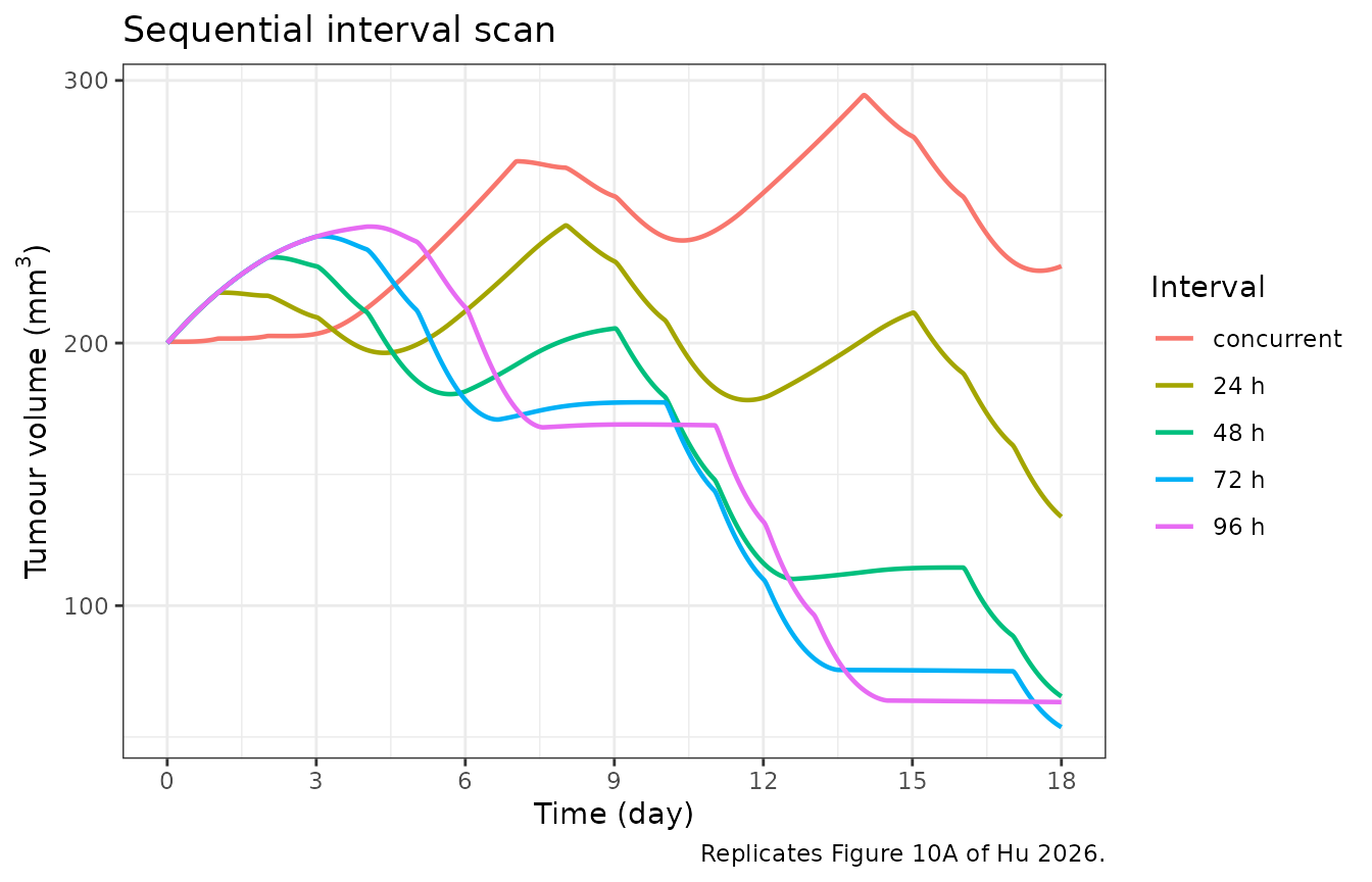
iv18 <- interval_sim |>
  group_by(interval) |>
  slice_min(abs(time - 18), n = 1, with_ties = FALSE) |>
  ungroup() |>
  select(interval, tumor_vol) |>
  mutate(tumor_vol = round(tumor_vol, 1)) |>
  rename(Interval = interval, `Day-18 tumour volume (mm3)` = tumor_vol)
knitr::kable(iv18, caption = "Day-18 tumour volume by sequential interval (Hu 2026 Figure 10A).")| Interval | Day-18 tumour volume (mm3) |
|---|---|
| concurrent | 229.3 |
| 24 h | 133.8 |
| 48 h | 65.4 |
| 72 h | 53.7 |
| 96 h | 63.3 |
v <- setNames(iv18$`Day-18 tumour volume (mm3)`, as.character(iv18$Interval))
stopifnot(
  # "less than half of that simulated with the 24 h interval"
  v[["48 h"]] < 0.5 * v[["24 h"]],
  # "extending the interval to 72 h or 96 h offered negligible additional benefits"
  abs(v[["72 h"]] / v[["48 h"]] - 1) < 0.25,
  abs(v[["96 h"]] / v[["48 h"]] - 1) < 0.25,
  # every sequential schedule beats concurrent dosing
  all(v[c("24 h", "48 h", "72 h", "96 h")] < v[["concurrent"]])
)
The mechanism behind the interval scan is visible in the intermediate states: the damaged-cell fraction plateaus by about 48 h after the first pemetrexed dose, so waiting longer adds nothing, while giving osimertinib early keeps a large fraction of cells arrested in the proliferating compartment where pemetrexed cannot damage them.
interval_sim |>
  filter(interval %in% c("concurrent", "24 h", "48 h")) |>
  select(time, interval, `Damaged cells (fraction)` = damaged_frac,
         `X1 / G1-arrested (fraction)` = x1_fraction,
         `EGFR signal (fraction of baseline)` = egfr_signal) |>
  pivot_longer(-c(time, interval), names_to = "state", values_to = "value") |>
  ggplot(aes(time, value, colour = interval)) +
  geom_line(linewidth = 0.7) +
  facet_wrap(~state, ncol = 1, scales = "free_y") +
  scale_x_continuous(breaks = seq(0, 18, by = 3)) +
  labs(x = "Time (day)", y = NULL, colour = "Interval",
       caption = "Replicates Figure 10C,E of Hu 2026 plus the EGFR state driving them.") +
  theme_bw()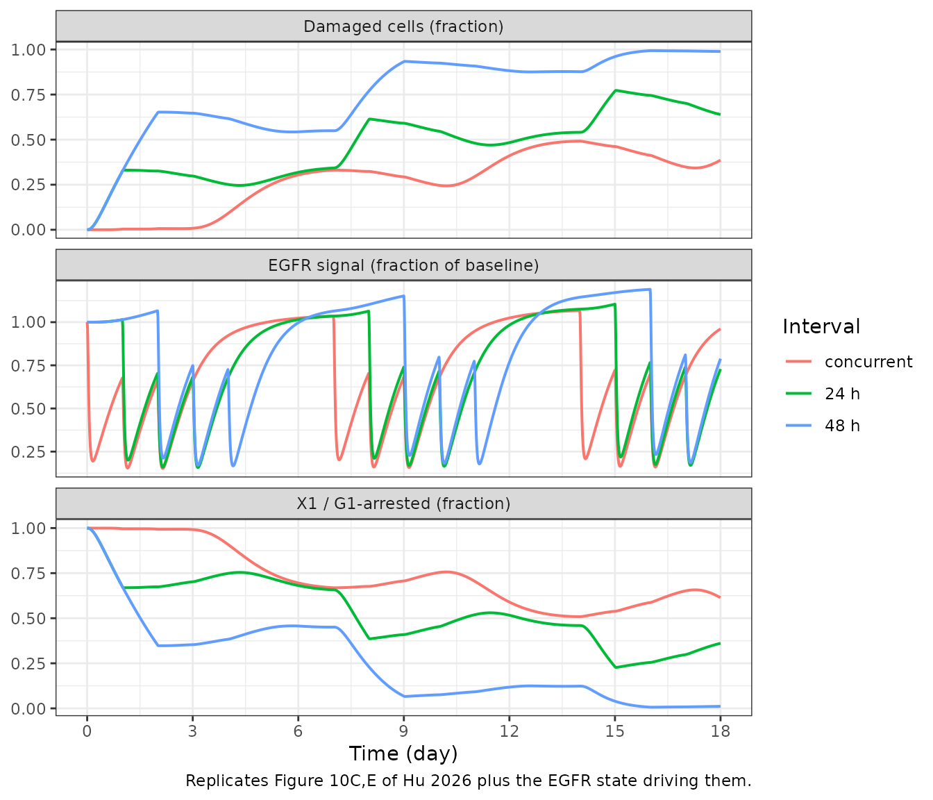
Replicates Figure 10C,E of Hu 2026: damaged-cell and X1 fractions.
# Hu 2026 Figure 10C: the 48 h schedule reaches a substantially higher damaged
# fraction than either the concurrent regimen or the 24 h interval.
peak_damaged <- interval_sim |>
  group_by(interval) |>
  summarise(peak = max(damaged_frac), .groups = "drop")
knitr::kable(peak_damaged |>
               mutate(peak = round(peak, 3)) |>
               rename(Interval = interval, `Peak damaged-cell fraction` = peak),
caption = "Peak damaged-cell fraction by schedule (Hu 2026 Figure 10C).")| Interval | Peak damaged-cell fraction |
|---|---|
| concurrent | 0.492 |
| 24 h | 0.773 |
| 48 h | 0.994 |
| 72 h | 1.000 |
| 96 h | 1.000 |
pk <- setNames(peak_damaged$peak, as.character(peak_damaged$interval))
stopifnot(pk[["48 h"]] > pk[["24 h"]], pk[["24 h"]] > pk[["concurrent"]])
Replicating Figure 11: Monte Carlo objective response rate
Hu 2026 Section 3.6 generates virtual tumour-bearing mice by applying
30% CV log-normal variability to every pharmacodynamic and tumour-growth
parameter and by drawing a BIM-deletion genotype with 11.5% prevalence
(CTONG0901); in the deleted genotype k_bim falls to 21.1
and gamma_bim rises five-fold. A responder is a subject
whose tumour volume falls to 70% or less of its starting value (RECIST
1.1), and the objective response rate (ORR) is followed over 210 days –
30 treatment cycles.
The 30% CV variability is already encoded in the model as fixed eta variances, so only the genotype needs to be applied here. Rather than drawing a genotype per subject, each genotype is simulated as its own cohort of 200 animals and the two are combined with the published 88.5% / 11.5% weights; this gives the same population ORR with far less Monte Carlo noise at this cohort size.
n_mc      <- 200L              # per cohort; 4 cohorts = 2 strategies x 2 genotypes
mc_cycles <- seq(0, by = 7, length.out = 30L)
mc_pem    <- sort(as.vector(outer(pem_hours,
                                  as.vector(outer(mc_cycles, pem_days, "+")), "+")))
mc_conc   <- sort(as.vector(outer(mc_cycles, c(0, 1, 2), "+")))
mc_seq    <- sort(as.vector(outer(mc_cycles, c(2, 3, 4), "+")))

mc_events <- list(
  "PEM + OSI"  = make_events(pem = mc_pem, osi = mc_conc,
                             obs = seq(0, 210, by = 1), n = n_mc),
  "PEM -> OSI" = make_events(pem = mc_pem, osi = mc_seq,
                             obs = seq(0, 210, by = 1), n = n_mc)
)
genotype <- list(
  "BIM wild type" = ui,
  "BIM deletion"  = rxode2::ini(ui, lkbim = log(21.1), lgamma_bim = log(0.595 * 5))
)
#> ℹ change initial estimate of `lkbim` to `3.04927304048202`
#> ℹ change initial estimate of `lgamma_bim` to `1.09024403899759`
genotype_weight <- c("BIM wild type" = 0.885, "BIM deletion" = 0.115)

mc <- list()
for (gn in names(genotype)) {
  for (an in names(mc_events)) {
    # Reseed inside the loop so every cohort draws the same etas (common
    # random numbers), which removes the between-arm sampling noise.
    rxode2::rxSetSeed(1042)
    s <- as.data.frame(rxode2::rxSolve(genotype[[gn]], mc_events[[an]],
                                       atol = 1e-8, rtol = 1e-8))
    mc[[paste(gn, an)]] <- tibble::tibble(id = s$id, time = s$time,
                                          tumor_vol = s$tumor_vol,
                                          genotype = gn, arm = an)
  }
}
mc <- bind_rows(mc)
stopifnot(all(is.finite(mc$tumor_vol)))

orr_curve <- mc |>
  group_by(arm, genotype, time) |>
  summarise(responder = mean(tumor_vol <= 0.70 * 200), .groups = "drop") |>
  group_by(arm, time) |>
  summarise(orr = 100 * sum(responder * genotype_weight[genotype]), .groups = "drop")
ggplot(orr_curve, aes(time, orr, colour = arm)) +
  geom_line(linewidth = 0.9) +
  scale_x_continuous(breaks = seq(0, 210, by = 30)) +
  labs(x = "Time (day)", y = "Simulated ORR (%)", colour = NULL,
       title = "Objective response rate, 2000-mouse design scaled to 200 per cohort",
       caption = "Replicates Figure 11C of Hu 2026.") +
  theme_bw()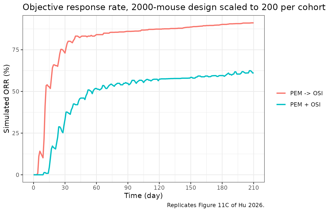
Replicates Figure 11C of Hu 2026: simulated ORR over 210 days.
orr_end <- orr_curve |>
  filter(time == 210) |>
  mutate(Published = c(67.14, 91.6)[match(arm, c("PEM + OSI", "PEM -> OSI"))],
         orr = round(orr, 1)) |>
  rename(Arm = arm, `Simulated ORR at day 210 (%)` = orr,
         `Hu 2026 Figure 11C (%)` = Published) |>
  select(-time)
knitr::kable(orr_end, caption = "Simulated versus published objective response rate.")| Arm | Simulated ORR at day 210 (%) | Hu 2026 Figure 11C (%) |
|---|---|---|
| PEM + OSI | 61.1 | 67.14 |
| PEM -> OSI | 92.3 | 91.60 |
o <- setNames(orr_end$`Simulated ORR at day 210 (%)`, as.character(orr_end$Arm))
stopifnot(
  # The paper's central population-level claim.
  o[["PEM -> OSI"]] - o[["PEM + OSI"]] > 15,
  # Agreement with Figure 11C. The band is wide enough to absorb Monte Carlo
  # error at 200 per cohort (standard error about 3 percentage points) and any
  # change in the rxode2 eta sampler across versions.
  abs(o[["PEM -> OSI"]] - 91.6)  < 15,
  abs(o[["PEM + OSI"]]  - 67.14) < 15
)
Assumptions and deviations
-
Pemetrexed peripheral transfer. Supplementary Table
S17 row 10 writes the pemetrexed distribution flux as
(k12*C1 - k21*C2) * PEM_V1, i.e. it scales the return term by the central volume. Printed Equations (2)-(3), the corresponding osimertinib row of Table S17, and the fact that the parameters came from a WinNonlin two-compartment fit all give the standard amount-balanced formk12*X1 - k21*X2. The standard form is implemented here. The two readings differ only by the factorV1/V2 = 1.21onk21and are numerically indistinguishable on the timescale of Figure S4A. -
Osimertinib bioavailability. Printed Equations
(4)-(5) carry an explicit
Fa,osion the absorption term, but no value forFa,osiis tabulated and Table S19 reports the volumes as the apparentOSI_V1/FandOSI_V2/F. Table S17 rows 15-16, the ODE export of the implemented model, carries noFaterm. The apparent-parameter form (no explicitF, volumes areV/F) is implemented. -
Damaged-cell fraction scale. Printed Equation (15)
writes
Damaged% = (X2+X3+X4)/(X1+X2+X3+X4) x 100%, but Table S18 row 3 and Table S20 both define it as the bare ratio with initial value 0 and unit “unitless”. The fraction is implemented. Feeding a percentage into the EGFR feedback term withk_EGFR_feedback = 0.2andgamma_EGFR_feedback = 1.45would raise baseline EGFR roughly a hundredfold, which is not what any figure in the paper shows. -
Clamp on the Bim term. The apoptosis term
1 + k_bim * (1 - EGFR)^gamma_bimhasgamma_bim = 0.595, a non-integer exponent, and was fitted (Figure 7L) over EGFR levels below baseline. Whenever osimertinib is absent the damaged-cell feedback lifts EGFR above 1, making the base negative and the power undefined; the published equation returnsNaNwithin the first solver step of every arm, including the untreated control. The deviation is therefore clamped at zero (max(1 - EGFR, 0)), so above baseline there is no Bim induction and no acceleration – the only reading that is both defined and consistent with the biology the paper describes. - Guard on the damaged-cell fraction denominator. In the 210-day Monte Carlo the most responsive virtual animals drive the tumour to about 1e-24 mm^3, where solver round-off pushes the states through zero and the ratio becomes 0/0. The denominator is floored at 1e-12 mm^3 and the numerator at zero. A single tumour cell is of order 1e-6 mm^3, so the guard cannot engage at any physically meaningful volume.
-
Untreated control is not identical to its drug-free
twin. Table S17 rows 5-8 define the unperturbed chain with no
EGFR terms at all, while the perturbed chain multiplies proliferation by
EGFR^gamma_EGFR. Because damaged-cell feedback lifts EGFR to about 1.015 even without drug, the untreated control grows a few percent faster than its own reference, giving a small negative TGI. This is a property of the published model, not of the transcription; the structural check above bounds it at 5%. -
Between-subject variability. Supplementary Method
S1.7 states that “all other PD parameters and tumour growth-related
parameters were also assigned 30% log-normally distributed
inter-individual variability”. Etas with the prescribed fixed variance
ln(1 + 0.30^2)are therefore placed on all 21 pharmacodynamic and tumour-growth parameters. Two quantities are excluded: the Simeoni switching exponentpsi, which is a numerical smoothing exponent taken from Simeoni 2004 rather than a biological parameter, and the baseline tumour volume, which Method S1.7 does not list among the varied quantities. No eta is placed on the pharmacokinetic parameters – the mouse PK was fitted to pooled mean profiles, so no individual PK variability is reported. -
BIM-deletion genotype is a simulation scenario, not a
covariate. Hu 2026 builds one model with one parameter set and
no covariate effects; the BIM-deletion analysis of Figure 11 and the
reduced-OSI-sensitivity analyses of Figure 9 substitute typical values
(
k_bimx 0.1 andgamma_bimx 5;EC50_osix 5,Imax_osi/ 5). Those are reproduced here by overriding the typical values withrxode2::ini()rather than by adding a covariate to the model file, which keepscovariateDataempty exactly as the paper’s model is. - Monte Carlo cohort size. Hu 2026 simulated 2000 virtual mice. This vignette uses 200 per cohort (the package cap), with the two genotypes run as separate cohorts and combined at the published 88.5% / 11.5% weights, and widens the ORR acceptance band accordingly.
-
Residual error. Hu 2026 reports no residual-error
model: the QSP model is calibrated against mean tumour volumes and used
for simulation. The tumour endpoint therefore carries
propSd_tumor_vol <- fixed(0); a user fitting the model to individual data should re-estimate it. - Dosing schedule read from a figure. The per-cycle dosing days are read from the schematic in Hu 2026 Figure 6A (pemetrexed on days 0-1; osimertinib on days 0-2 concurrent or days 2-4 sequential, 7-day cycle). Figures S4C-F, which plot the simulated concentration-time profiles under exactly that schedule, confirm the reading: the dose spikes fall on the same days and the simulated peaks reproduce the published axes.
- Peak-concentration references. The 42 mg/L and 57 ug/L reference peaks used in the Cmax comparison are read from the y-axes of Hu 2026 Figures S4C and S4D, which are the paper’s own simulated profiles; the AUC and half-life references are closed-form from the Table S19 micro-constants and involve no figure reading.