Pemigatinib population PK and exposure-response (Gong 2023)
Source:vignettes/articles/Gong_2023_pemigatinib.Rmd
Gong_2023_pemigatinib.RmdModel and source
Gong 2023 reports two things: a refined population PK model for pemigatinib, and a set of exposure-response analyses built on top of it. Three of those models are packaged here.
- Citation: Gong X, Akil A, Ndi A, Ji T, Liu X, Lovern M, Chen X. (2023). Population pharmacokinetic and exposure-response analyses of pemigatinib in patients with advanced solid tumors including cholangiocarcinoma. CPT Pharmacometrics Syst Pharmacol 12(11):1784-1794. doi:10.1002/psp4.13064
- Article: https://doi.org/10.1002/psp4.13064
- Supplement (Appendix S1, containing Table S1, Table S2 and the final NONMEM control stream): https://doi.org/10.1002/psp4.13064
| Model | Role |
|---|---|
Gong_2023_pemigatinib |
Two-compartment population PK with sequential zero-/first-order absorption |
Gong_2023_pemigatinib_phosphate |
Direct-effect Emax model for the change from baseline in serum phosphate, driven by steady-state AUC and baseline phosphate |
Gong_2023_pemigatinib_creatinine |
Direct-effect Emax model for percentage change from baseline in serum creatinine, driven by steady-state AUC |
mod  <- readModelDb("Gong_2023_pemigatinib")
modp <- readModelDb("Gong_2023_pemigatinib_phosphate")
modc <- readModelDb("Gong_2023_pemigatinib_creatinine")
Pemigatinib is a selective inhibitor of fibroblast growth factor receptor (FGFR) 1-3, approved for previously treated, unresectable locally advanced or metastatic cholangiocarcinoma (CCA) with FGFR2 fusions or rearrangements, and for relapsed/refractory myeloid/lymphoid neoplasms with FGFR1 rearrangement. The recommended regimen is 13.5 mg orally once daily on a 21-day cycle, 2 weeks on and 1 week off.
Population
The population PK analysis pooled 4552 concentration records from 467 healthy participants and patients across seven FIGHT studies (FIGHT-101, -102, -104, -105, -106, -202, -203; Gong 2023 Table S1). Mean (SD) age was 54.3 (14.5) years with a median of 56 and range 19-83; mean (SD) baseline body weight was 75.7 (19.7) kg with a median of 73.9 kg and range 39.8-156 kg; 219 of 467 (46.9%) were men, so women are the more common – and therefore reference – sex category. Tumour types were CCA (163; 34.9%), myeloid/lymphoid neoplasms with FGFR1 rearrangement (34; 7.3%), other cancers (192; 41.1%), and healthy participants (78; 16.7%). Relevant co-medication use was phosphate binders in 61 (13.1%), proton-pump inhibitors (PPI) in 114 (24.4%), and histamine-2 receptor antagonists (H2RA) in 39 (8.4%). 89.3% received pemigatinib monotherapy. Baseline demographics are Gong 2023 Table 1.
Both serum-chemistry exposure-response analyses – serum phosphate and serum creatinine – used the same 300 monotherapy patients pooled from FIGHT-101, FIGHT-102, and FIGHT-202. The objective-response analyses used the 108 patients with CCA carrying FGFR2 fusions or rearrangements.
The same information is available programmatically via
readModelDb("Gong_2023_pemigatinib")()$population.
Source trace
Per-parameter origins are recorded as in-file comments next to each
ini() entry in
inst/modeldb/specificDrugs/Gong_2023_pemigatinib.R and
inst/modeldb/specificDrugs/Gong_2023_pemigatinib_creatinine.R.
They are collected here for review.
Population PK model
| Equation / parameter | Value | Source location |
|---|---|---|
lcl (CL/F) |
10.7 L/h | Table 2, %RSE 2.7, 95% CI 10.1-11.3 |
lvc (Vc/F) |
118 L | Table 2, %RSE 3.4, 95% CI 110-125 |
lvp (Vp/F) |
95.0 L | Table 2, %RSE 3.0, 95% CI 89.4-101 |
lq (Q/F) |
25.2 L/h | Table 2, %RSE 7.7, 95% CI 21.4-29.0 |
lka (ka) |
3.67 1/h | Table 2, %RSE 12.2, 95% CI 2.79-4.55 |
ld1 (D1) |
0.810 h | Table 2, %RSE 3.0, 95% CI 0.763-0.857 |
e_phosbinder_cl |
-0.155 | Table 2 “Phosphate binder on CL/F, %” = -15.5% |
e_male_cl |
+0.262 | Table 2 “Male sex on CL/F, %” = +26.2% |
e_ppi_ka |
-0.620 | Table 2 “PPI on Ka, %” = -62.0% |
e_male_ka |
-0.583 | Table 2 “Male sex on Ka, %” = -58.3% |
e_h2ra_d1 |
-0.334 | Table 2 “H2B antagonist on D1, %” = -33.4% |
e_wt_vc |
0.842 | Table 2; Appendix S1
V2BWT = ((BWT/73.9)**THETA(12))
|
e_wt_vp |
1.13 | Table 2; Appendix S1
V3BWT = ((BWT/73.9)**THETA(13))
|
| Reference weight | 73.9 kg | Appendix S1 control stream; = Table 1 cohort median |
etalcl, etalvc block |
0.200704, 0.129, 0.190969 | Table 2 IIV 44.8 / 43.7 %CV; covariance 0.129 from Table 2 footnote a |
etalka |
1.69 | Table 2 IIV Ka 130 %CV |
etald1 |
0.370881 | Table 2 IIV D1 60.9 %CV |
| IIV on Q/F, Vp/F | fixed to 0 | Table 2 “Fixed to 0”; Appendix S1 $OMEGA 0 FIX
|
propSd |
0.323 | Table 2 RUV 32.3%; Appendix S1 $ERROR log-additive |
| Absorption structure | sequential zero-order D1 then first-order ka | Appendix S1 $SUBROUTINE ADVAN4 TRANS4 with
D1=TVD1*EXP(ETA(6)); Results paragraph 2 |
Cc unit conversion |
x 1e6 / 487.5 |
Appendix S1 S2 = V2/1000000*487.5 ;nM (pemigatinib MW
487.5 g/mol) |
Serum-phosphate exposure-response model
| Equation / parameter | Value | Source location |
|---|---|---|
lemax |
5.51 mg/dL | Table S2, approximate SE 0.368, 95% CL 4.79-6.23 |
lec50 |
1665 h*nM | Table S2, approximate SE 357, 95% CL 963-2367 |
e_phos_base |
-0.185 per mg/dL, carried as -0.5730 per mmol/L | Table S2, approximate SE 0.0812, 95% CL -0.345 to -0.0250; rescaled by 3.0975 mg/dL per mmol/L |
phosChange = Emax * AUC / (EC50 + AUC) + coef * PHOS |
n/a | Methods “Exposure-response evaluation”; additive form confirmed by the Results sentence quoted below |
| Baseline phosphate is a covariate | n/a | Methods: “Serum phosphate at baseline was entered into the model as a covariate” |
| Residual error | not reported | absent from Table S2 and main text; encoded
fixed(0)
|
Serum-creatinine exposure-response model
| Equation / parameter | Value | Source location |
|---|---|---|
lemax |
43.4 % | Table S2, approximate SE 6.15, 95% CL 31.3-55.5 |
lec50 |
2595 h*nM | Table S2, approximate SE 793, 95% CL 1035-4154 |
creatPctChange = Emax * AUC / (EC50 + AUC) |
n/a | Methods “Exposure-response evaluation” |
| Residual error | not reported | absent from Table S2 and main text; encoded
fixed(0)
|
Interpreting the reported %CV as a log-scale SD
Gong 2023 Table 2 reports inter-individual variability as “%CV”
without saying whether those numbers are 100 * omega (the
log-scale SD) or 100 * sqrt(exp(omega^2) - 1) (the
log-normal coefficient of variation). The paper’s own numbers settle it:
Table 2 gives the CL/F-Vc/F correlation as 0.659, and the footnote gives
the covariance as 0.129. Only one reading reproduces that
correlation.
cv_cl <- 0.448  # Table 2 IIV CL/F 44.8 %CV
cv_vc <- 0.437  # Table 2 IIV Vc/F 43.7 %CV
cov_cl_vc <- 0.129  # Table 2 footnote a

tibble::tibble(
  Reading = c("omega^2 = CV^2 (log-scale SD)", "omega^2 = log(1 + CV^2) (log-normal CV)"),
  `Implied correlation` = c(
    cov_cl_vc / (cv_cl * cv_vc),
    cov_cl_vc / sqrt(log(1 + cv_cl^2) * log(1 + cv_vc^2))
  ),
  `Reported (Table 2)` = 0.659
) |>
knitr::kable(digits = 4, caption = "The reported %CV values are log-scale SDs.")| Reading | Implied correlation | Reported (Table 2) |
|---|---|---|
| omega^2 = CV^2 (log-scale SD) | 0.6589 | 0.659 |
| omega^2 = log(1 + CV^2) (log-normal CV) | 0.7215 | 0.659 |
The Appendix S1 $OMEGA initial estimates corroborate the
same reading: the ka initial 1.65573 has square root 1.287 (128.7%)
against the 130% final, and the D1 initial 0.429359 has square root
0.655 (65.5%) against the 60.9% final. The model file therefore encodes
omega^2 = CV^2.
Virtual cohort
Original observed data are not publicly available. The stochastic simulation below uses a virtual population whose body-weight distribution approximates the published trial demographics (Gong 2023 Table 1): drawn log-normally with a median of 73.9 kg and truncated to the observed 39.8-156 kg range. All other covariates are set to the reference level (female, no concomitant phosphate binder, proton-pump inhibitor, or H2-receptor antagonist).
Covariate effects are examined separately, in the
typical-value section further down, because Gong 2023 states
its own co-medication results as typical-subject simulations. A
deterministic comparison isolates the published coefficients exactly; a
stochastic one would only add sampling noise, and with 130% CV on
ka that noise is large.
set.seed(20231101)

n_subj <- 200L
dose_mg <- 13.5
n_days <- 8L  # terminal t1/2 is ~15 h, so 8 days is >12 half-lives to steady state
tau <- 24
ss_start <- (n_days - 1) * tau

subj <- tibble::tibble(
  id = seq_len(n_subj),
  WT = pmin(pmax(rlnorm(n_subj, meanlog = log(73.9), sdlog = 0.25), 39.8), 156),
  SEXF = 1,
  CONMED_PPI = 0,
  CONMED_H2RA = 0,
  CONMED_PHOSBINDER = 0
)

doses <- subj |>
  tidyr::crossing(time = seq(0, by = tau, length.out = n_days)) |>
  dplyr::mutate(
    amt = dose_mg,
    evid = 1L,
    # rate = -2 tells rxode2 to apply the model's dur(depot) zero-order window
    # rather than treating the dose as an instantaneous bolus.
    rate = -2,
    cmt = "depot"
  )

obs <- subj |>
  tidyr::crossing(time = ss_start + seq(0, tau, by = 0.25)) |>
  dplyr::mutate(
    amt = NA_real_,
    evid = 0L,
    rate = NA_real_,
    # Observations sit on the ODE state, never on the algebraic observable Cc
    # (which would auto-inject a cmt slot and renumber the states).
    cmt = "central"
  )

events <- dplyr::bind_rows(doses, obs) |>
  dplyr::arrange(id, time, dplyr::desc(evid))

stopifnot(!anyDuplicated(unique(events[, c("id", "time", "evid")])))
Simulation
sim <- rxode2::rxSolve(mod, events = events, keep = c("WT")) |>
  as.data.frame()
#> ℹ parameter labels from comments will be replaced by 'label()'
Replicate published figures
Steady-state concentration-time profile (structure of Figure 1)
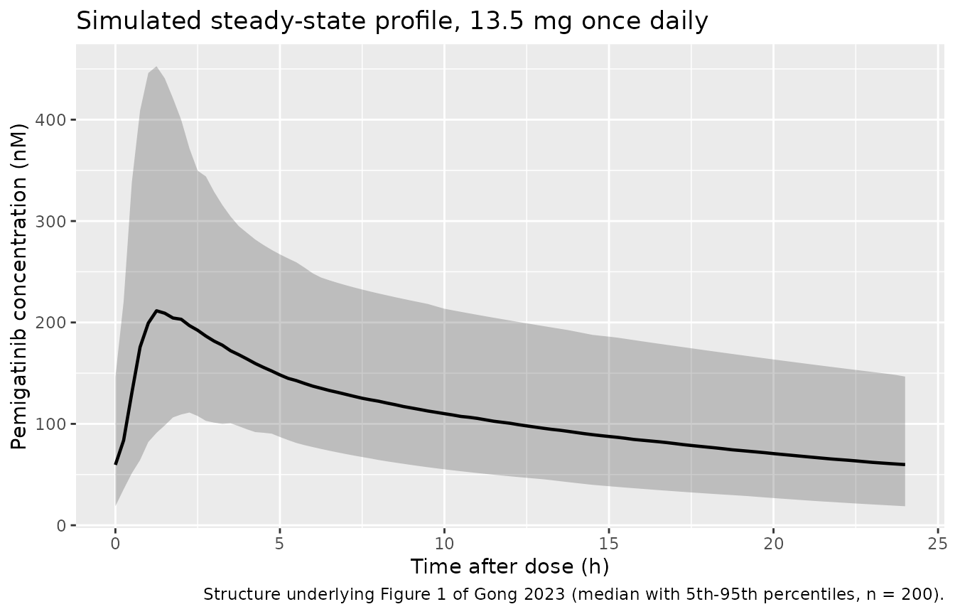
Gong 2023 Figure 1 is a prediction-corrected and an ordinary visual
predictive check over the whole pooled dataset. The published figure
cannot be reproduced without the observed data, but the simulated median
and 5th/95th percentiles over a steady-state interval at the recommended
13.5 mg once-daily dose show the behaviour the model encodes: a
zero-order release window of D1 followed by rapid
first-order absorption, and a biphasic decline.
sim |>
  dplyr::mutate(tad = time - ss_start) |>
  dplyr::group_by(tad) |>
  dplyr::summarise(
    Q05 = quantile(Cc, 0.05),
    Q50 = quantile(Cc, 0.50),
    Q95 = quantile(Cc, 0.95),
    .groups = "drop"
  ) |>
  ggplot(aes(tad, Q50)) +
  geom_ribbon(aes(ymin = Q05, ymax = Q95), alpha = 0.25) +
  geom_line(linewidth = 0.8) +
  labs(
    x = "Time after dose (h)", y = "Pemigatinib concentration (nM)",
    title = "Simulated steady-state profile, 13.5 mg once daily",
    caption = "Structure underlying Figure 1 of Gong 2023 (median with 5th-95th percentiles, n = 200)."
  )
Serum phosphate vs steady-state exposure (Figure 2)
Gong 2023 Figure 2 plots the model-predicted mean change from
baseline in serum phosphate at C1D8/C1D15 against steady-state AUC. The
published parameters are in the paper’s mg/dL, but the canonical
covariate column PHOS is SI mmol/L, so the baseline
coefficient is carried rescaled. The two units are related by the atomic
mass of elemental phosphorus.
MGDL_PER_MMOLL <- 30.974 / 10  # elemental phosphorus, 30.974 g/mol; 1 mmol/L = 3.0975 mg/dL
auc_ref_135 <- 2850            # Gong 2023 Results: mean AUCss at 13.5 mg q.d.
Baseline serum phosphate is not tabulated by Gong 2023, so the curve is drawn as a band spanning the adult clinical reference range, 2.5-4.5 mg/dL.
phos_grid <- tidyr::crossing(
  AUC_PEMI = seq(0, 9000, length.out = 100),
  PHOS_mgdL = c(2.5, 3.5, 4.5)
) |>
  dplyr::mutate(
    id = dplyr::row_number(),
    time = 0,
    PHOS = PHOS_mgdL / MGDL_PER_MMOLL
  )

phos_sim <- rxode2::rxSolve(modp, events = phos_grid,
                            keep = c("AUC_PEMI", "PHOS_mgdL")) |>
  as.data.frame()
#> Warning: multi-subject simulation without without 'omega'

ggplot(phos_sim, aes(AUC_PEMI, phosChange, group = PHOS_mgdL,
                     linetype = factor(PHOS_mgdL))) +
  geom_line(linewidth = 0.8) +
  geom_vline(xintercept = 1665, colour = "firebrick", linetype = "dotted") +
  labs(
    x = "Steady-state AUC (h*nM)",
    y = "Change from baseline in serum phosphate (mg/dL)",
    linetype = "Baseline phosphate (mg/dL)",
    title = "Serum phosphate exposure-response",
    caption = paste(
      "Replicates Figure 2 of Gong 2023. The dotted line is the fitted",
      "EC50 of 1665 h*nM, which the paper notes approximates the mean",
      "AUC0-24h at 8 mg once daily."
    )
  ) +
  theme(legend.position = "bottom")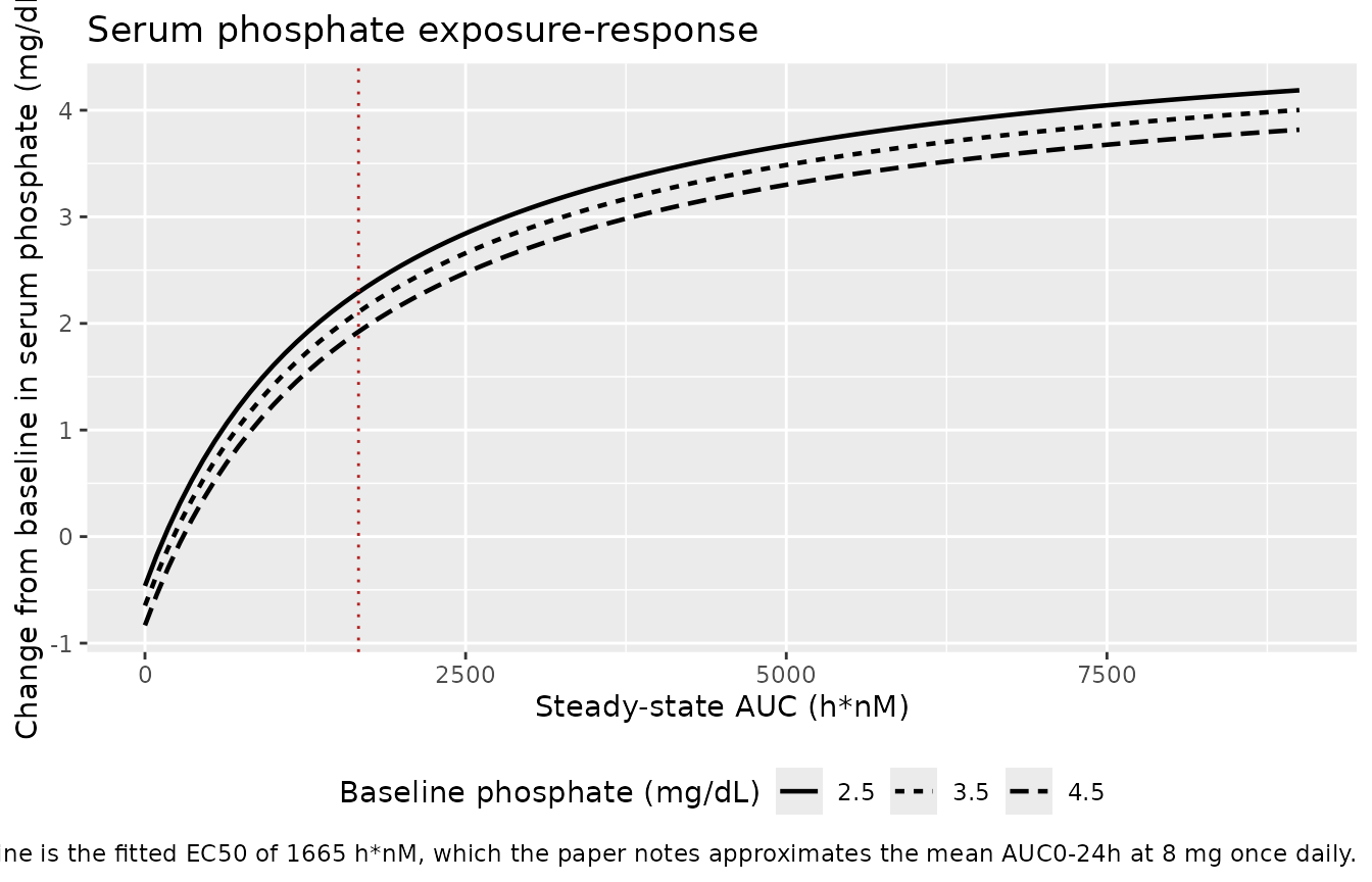
The baseline covariate enters additively, not multiplicatively
Table S2 labels the baseline coefficient (mg/dL)^-1,
which reads as an inverse-concentration unit and would suggest a
multiplicative form Emax * E(AUC) * (1 + coef * PHOS). The
paper’s own Results sentence settles it in favour of the additive form:
“For every 1-mg/dL increase in baseline serum phosphate level, the
reduction from baseline was less than or equal to 0.185 mg/dL”. A
constant absolute offset per unit of baseline, independent of exposure,
is the additive reading; under the multiplicative reading the offset
would scale with the Emax term. The two forms are far apart numerically
at the recommended dose, and only the additive one lands near the
paper’s reported median change of about 2.7 mg/dL.
phos_base <- 3.5  # mid-normal-range assumption; see Assumptions and deviations
emax_p <- 5.51
ec50_p <- 1665
e_drug <- emax_p * auc_ref_135 / (ec50_p + auc_ref_135)

tibble::tibble(
  Form = c("Additive (packaged)", "Multiplicative (rejected)"),
  Equation = c("Emax * E + coef * PHOS", "Emax * E * (1 + coef * PHOS)"),
  `Predicted change at 13.5 mg (mg/dL)` = c(
    e_drug - 0.185 * phos_base,
    e_drug * (1 - 0.185 * phos_base)
  ),
  `Observed median (mg/dL)` = 2.7
) |>
  knitr::kable(digits = 2,
caption = "Only the additive form reproduces the reported median change.")| Form | Equation | Predicted change at 13.5 mg (mg/dL) | Observed median (mg/dL) |
|---|---|---|---|
| Additive (packaged) | Emax * E + coef * PHOS | 2.83 | 2.7 |
| Multiplicative (rejected) | Emax * E * (1 + coef * PHOS) | 1.23 | 2.7 |
Gates
Three checks: the EC50 half-maximal identity, the unit-conversion round trip, and the paper’s observed median change from baseline.
eval_phos <- function(auc, phos_mgdL) {
  ev <- tibble::tibble(
    id = seq_along(auc),
    time = 0,
    AUC_PEMI = auc,
    PHOS = phos_mgdL / MGDL_PER_MMOLL
  )
  rxode2::rxSolve(modp, events = ev)$phosChange
}

# 1. At AUC = EC50 with a zero baseline term, the drug effect is exactly Emax/2.
half_max <- eval_phos(1665, 0)

# 2. Unit-conversion round trip: raising baseline phosphate by 1 mg/dL must lower
#    the predicted change by exactly the published 0.185 mg/dL, even though the
#    model is driven by an SI mmol/L column and a rescaled coefficient.
slope_per_mgdL <- diff(eval_phos(c(auc_ref_135, auc_ref_135), c(3.0, 4.0)))
#> Warning: multi-subject simulation without without 'omega'

# 3. Median change from baseline. Gong 2023 Figure 3b gives the median AUCss in
#    the CCA efficacy population as the second/third quartile boundary, 2351
#    h*nM; Figure 3a gives the median change from baseline as the corresponding
#    boundary, 2.7 mg/dL. Driving the model at that exposure across the adult
#    reference range for baseline phosphate must bracket the observed median.
med_band <- eval_phos(c(2351, 2351), c(2.5, 4.5))
#> Warning: multi-subject simulation without without 'omega'

tibble::tibble(
  Check = c("Emax/2 at AUC = EC50 (mg/dL)",
            "Change per +1 mg/dL baseline (mg/dL)",
            "Predicted change at median AUCss, baseline 4.5 mg/dL",
            "Predicted change at median AUCss, baseline 2.5 mg/dL"),
  Model = c(half_max, slope_per_mgdL, med_band[2], med_band[1]),
  Published = c(5.51 / 2, -0.185, NA, NA),
  Source = c("Table S2 Emax", "Results / Table S2 coefficient",
             "brackets the observed median of 2.7 (Figure 3a)",
             "brackets the observed median of 2.7 (Figure 3a)")
) |>
knitr::kable(digits = 4, caption = "Serum-phosphate model gates.")| Check | Model | Published | Source |
|---|---|---|---|
| Emax/2 at AUC = EC50 (mg/dL) | 2.7550 | 2.755 | Table S2 Emax |
| Change per +1 mg/dL baseline (mg/dL) | -0.1850 | -0.185 | Results / Table S2 coefficient |
| Predicted change at median AUCss, baseline 4.5 mg/dL | 2.3931 | NA | brackets the observed median of 2.7 (Figure 3a) |
| Predicted change at median AUCss, baseline 2.5 mg/dL | 2.7631 | NA | brackets the observed median of 2.7 (Figure 3a) |
Serum creatinine vs steady-state exposure (Figure 4)
Gong 2023 Figure 4 plots model-predicted percentage change from baseline in serum creatinine against steady-state AUC. The paper states the predicted values at four doses (Results, “Exposure-response analysis of safety”), obtained from the mean post hoc AUCss at 13.5 mg once daily and the dose-scaled means at the other doses.
# auc_ref_135 (the published mean AUCss at 13.5 mg q.d.) is defined above.
# A plotting grid for the algebraic exposure-response curve -- these are
# evaluation points, not virtual participants.
creat_curve <- tibble::tibble(
  id = seq_len(200),
  time = 0,
  AUC_PEMI = seq(0, 9000, length.out = 200)
)

creat_sim <- rxode2::rxSolve(modc, events = creat_curve, keep = "AUC_PEMI") |>
  as.data.frame()
#> Warning: multi-subject simulation without without 'omega'

dose_points <- tibble::tibble(
  id = 1:4,
  time = 0,
  dose_mg = c(6, 9, 13.5, 20),
  AUC_PEMI = auc_ref_135 * c(6, 9, 13.5, 20) / 13.5
)

dose_pred <- rxode2::rxSolve(modc, events = dose_points, keep = c("AUC_PEMI", "dose_mg")) |>
  as.data.frame()
#> Warning: multi-subject simulation without without 'omega'

ggplot(creat_sim, aes(AUC_PEMI, creatPctChange)) +
  geom_line(linewidth = 0.8) +
  geom_point(data = dose_pred, aes(AUC_PEMI, creatPctChange),
             size = 2.5, colour = "firebrick") +
  labs(
    x = "Steady-state AUC (h*nM)",
    y = "Change from baseline in serum creatinine (%)",
    title = "Serum creatinine exposure-response",
    caption = "Replicates Figure 4 of Gong 2023; points are the 6, 9, 13.5 and 20 mg doses."
  )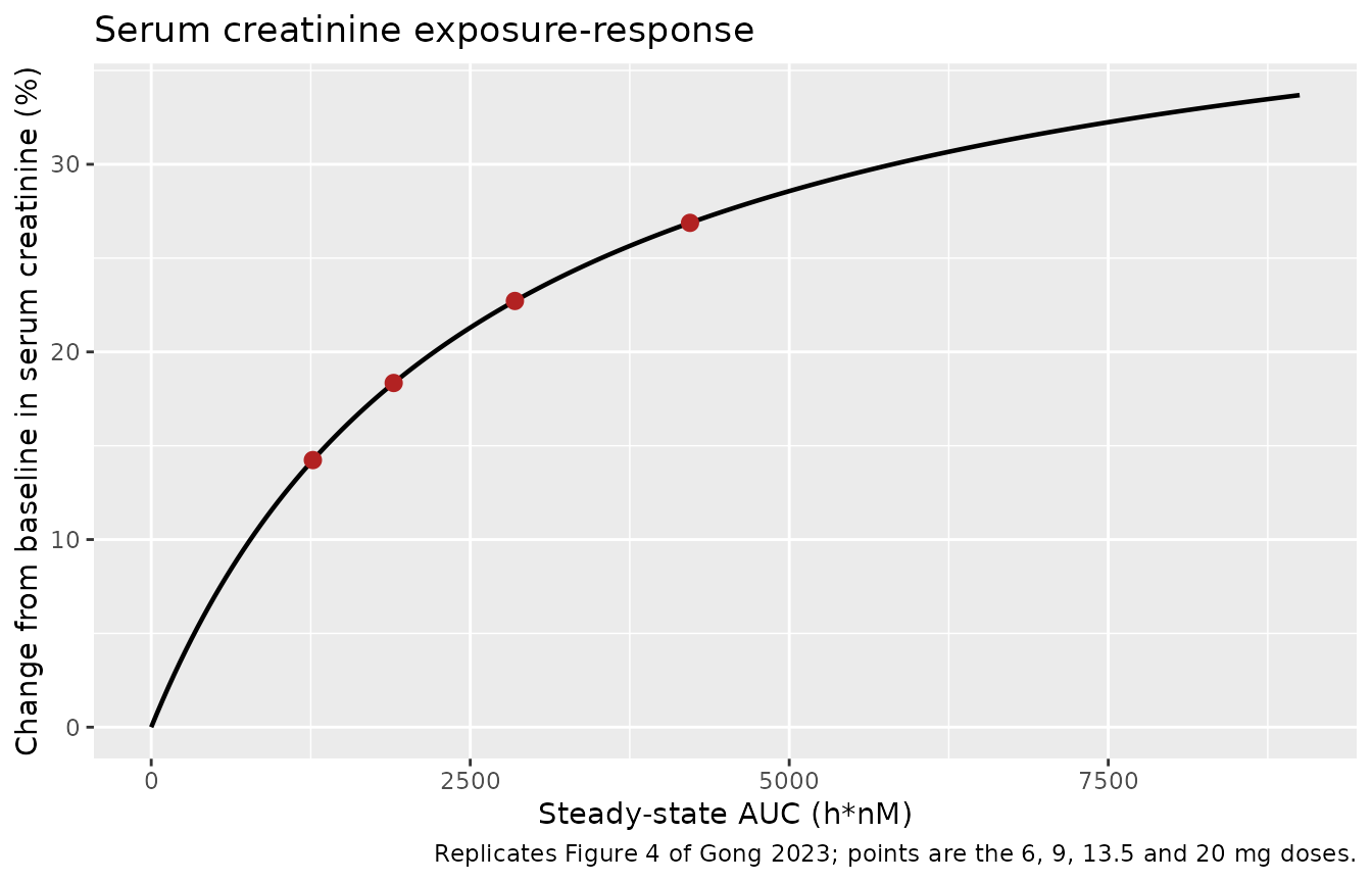
The four published predictions are reproduced exactly.
creat_cmp <- dose_pred |>
  dplyr::transmute(
    `Dose (mg)` = dose_mg,
    `AUCss (h*nM)` = round(AUC_PEMI, 1),
    Simulated = round(creatPctChange, 2),
    Published = c(14.2, 18.3, 22.7, 26.9)
  ) |>
  dplyr::mutate(`Difference (%)` = round(100 * (Simulated - Published) / Published, 2))

knitr::kable(
  creat_cmp,
  caption = "Serum creatinine percentage change: packaged model vs Gong 2023 Results."
)| Dose (mg) | AUCss (h*nM) | Simulated | Published | Difference (%) |
|---|---|---|---|---|
| 6.0 | 1266.7 | 14.24 | 14.2 | 0.28 |
| 9.0 | 1900.0 | 18.34 | 18.3 | 0.22 |
| 13.5 | 2850.0 | 22.72 | 22.7 | 0.09 |
| 20.0 | 4222.2 | 26.88 | 26.9 | -0.07 |
PKNCA validation
Noncompartmental parameters are computed over the final (steady-state) dosing interval.
sim_nca <- sim |>
  # Only !is.na(Cc): adding time > 0 or Cc > 0 would drop the anchor row PKNCA
  # needs at the interval start.
  dplyr::filter(!is.na(Cc)) |>
  dplyr::select(id, time, Cc) |>
  dplyr::mutate(regimen = "13.5 mg q.d.")

conc_obj <- PKNCA::PKNCAconc(sim_nca, Cc ~ time | regimen + id)

dose_df <- events |>
  dplyr::filter(evid == 1, time == ss_start) |>
  dplyr::select(id, time, amt) |>
  dplyr::mutate(regimen = "13.5 mg q.d.")

dose_obj <- PKNCA::PKNCAdose(dose_df, amt ~ time | regimen + id)

intervals <- data.frame(
  start = ss_start,
  end = ss_start + tau,
  cmax = TRUE,
  tmax = TRUE,
  cmin = TRUE,
  auclast = TRUE
)

nca_res <- PKNCA::pk.nca(PKNCA::PKNCAdata(conc_obj, dose_obj, intervals = intervals))

nca_tab <- as.data.frame(nca_res) |>
  # PKNCA emits dependency rows; restrict to the requested interval.
  dplyr::filter(start == ss_start, end == ss_start + tau) |>
  dplyr::filter(PPTESTCD %in% c("cmax", "tmax", "cmin", "auclast")) |>
  dplyr::select(regimen, id, PPTESTCD, PPORRES) |>
  tidyr::pivot_wider(names_from = PPTESTCD, values_from = PPORRES)

nca_tab |>
  dplyr::summarise(
    `Cmax,ss (nM)` = mean(cmax),
    `Cmin,ss (nM)` = mean(cmin),
    `AUCss (h*nM)` = mean(auclast),
    `Median Tmax (h)` = median(tmax)
  ) |>
  knitr::kable(digits = 1,
caption = "Simulated steady-state exposure, 13.5 mg once daily (n = 200).")| Cmax,ss (nM) | Cmin,ss (nM) | AUCss (h*nM) | Median Tmax (h) |
|---|---|---|---|
| 250.4 | 67 | 2897.2 | 1.5 |
Mean steady-state AUC at the recommended dose
Gong 2023 reports a mean AUCss of 2850 hnM at 13.5 mg once daily, and separately notes that the serum-phosphate EC50 of 1665 hnM “approximates the mean AUC0-24h from 8 mg q.d. pemigatinib”. Both are reproduced.
auc_mean <- mean(nca_tab$auclast)

auc_cmp <- tibble::tibble(
  Quantity = c("Mean AUCss at 13.5 mg", "Implied mean AUCss at 8 mg"),
  Simulated = c(auc_mean, auc_mean * 8 / 13.5),
  Published = c(2850, 1665),
  Source = c("Results, exposure-response of efficacy",
             "Results: phosphate EC50 1665 h*nM ~ 8 mg q.d.")
) |>
  dplyr::mutate(`Difference (%)` = 100 * (Simulated - Published) / Published)

knitr::kable(auc_cmp, digits = c(0, 0, 0, 0, 1),
caption = "Simulated vs published steady-state exposure anchors.")| Quantity | Simulated | Published | Source | Difference (%) |
|---|---|---|---|---|
| Mean AUCss at 13.5 mg | 2897 | 2850 | Results, exposure-response of efficacy | 1.7 |
| Implied mean AUCss at 8 mg | 1717 | 1665 | Results: phosphate EC50 1665 h*nM ~ 8 mg q.d. | 3.1 |
The arithmetic mean AUCss exceeds the typical-value AUCss because
clearance is log-normally distributed:
E[1/CL] = (1/CL_typical) * exp(omega^2 / 2), which for
omega^2 = 0.2007 inflates the mean by 10.6%.
Dose conservation
For the typical reference subject, AUCss over the dosing interval
must equal dose / (CL/F) converted to nM. This checks that
the sequential zero-/first-order absorption model loses no dose.
mod_typ <- rxode2::zeroRe(mod)
#> ℹ parameter labels from comments will be replaced by 'label()'

typ_events <- events |>
  dplyr::filter(id == 1L) |>
  dplyr::mutate(WT = 73.9)

sim_typ <- rxode2::rxSolve(mod_typ, events = typ_events) |>
  as.data.frame() |>
  dplyr::filter(time >= ss_start)
#> ℹ omega/sigma items treated as zero: 'etalcl', 'etalvc', 'etalka', 'etald1'

auc_trapz <- sum(diff(sim_typ$time) *
                   (head(sim_typ$Cc, -1) + tail(sim_typ$Cc, -1)) / 2)
auc_closed <- dose_mg / 10.7 * 1e6 / 487.5

tibble::tibble(
  `Simulated AUCss (h*nM)` = auc_trapz,
  `Closed form dose/(CL/F) (h*nM)` = auc_closed,
  `Difference (%)` = 100 * (auc_trapz - auc_closed) / auc_closed
) |>
  knitr::kable(digits = c(1, 1, 4),
caption = "Dose conservation through the sequential zero-/first-order absorption model.")| Simulated AUCss (h*nM) | Closed form dose/(CL/F) (h*nM) | Difference (%) |
|---|---|---|
| 2587.6 | 2588.1 | -0.0196 |
Typical-subject covariate effects
Gong 2023 Results states: “Simulated Cmax,ss values were 12% lower and 1.1% higher, respectively, in typical PPI or H2B users versus nonusers.” Because those are typical-value statements, they are reproduced deterministically with the random effects zeroed, at the cohort-median weight of 73.9 kg.
typ_profile <- function(sexf, ppi, h2ra, binder) {
  # A single deterministic subject, so a dense grid is cheap. The 0.25 h grid
  # used for the stochastic cohort is too coarse to resolve Cmax to the one
  # decimal place the paper reports.
  ev_dose <- events |> dplyr::filter(id == 1L, evid == 1L)
  ev_obs <- ev_dose[1, ] |>
    dplyr::select(id, amt, evid, rate, cmt) |>
    dplyr::mutate(amt = NA_real_, evid = 0L, rate = NA_real_, cmt = "central") |>
    tidyr::crossing(time = ss_start + seq(0, tau, by = 0.01))

  ev <- dplyr::bind_rows(ev_dose, ev_obs) |>
    dplyr::arrange(time, dplyr::desc(evid)) |>
    dplyr::mutate(
      WT = 73.9,
      # Lower-case argument names so the dplyr data mask cannot shadow them
      # with the same-named event-table columns.
      SEXF = sexf,
      CONMED_PPI = ppi,
      CONMED_H2RA = h2ra,
      CONMED_PHOSBINDER = binder
    )
  s <- rxode2::rxSolve(mod_typ, events = ev) |>
    as.data.frame() |>
    dplyr::filter(time >= ss_start)
  c(
    cmax = max(s$Cc),
    cmin = min(s$Cc),
    auc = sum(diff(s$time) * (head(s$Cc, -1) + tail(s$Cc, -1)) / 2)
  )
}

ref_t    <- typ_profile(1, 0, 0, 0)
#> ℹ omega/sigma items treated as zero: 'etalcl', 'etalvc', 'etalka', 'etald1'
male_t   <- typ_profile(0, 0, 0, 0)
#> ℹ omega/sigma items treated as zero: 'etalcl', 'etalvc', 'etalka', 'etald1'
ppi_t    <- typ_profile(1, 1, 0, 0)
#> ℹ omega/sigma items treated as zero: 'etalcl', 'etalvc', 'etalka', 'etald1'
h2ra_t   <- typ_profile(1, 0, 1, 0)
#> ℹ omega/sigma items treated as zero: 'etalcl', 'etalvc', 'etalka', 'etald1'
binder_t <- typ_profile(1, 0, 0, 1)
#> ℹ omega/sigma items treated as zero: 'etalcl', 'etalvc', 'etalka', 'etald1'

pct <- function(a, b, m) 100 * (a[m] / b[m] - 1)

typ_cmp <- tibble::tibble(
  Comparison = c("PPI user vs nonuser", "H2RA user vs nonuser",
                 "Phosphate-binder user vs nonuser", "Women vs men"),
  `Cmax,ss (%)` = c(pct(ppi_t, ref_t, "cmax"), pct(h2ra_t, ref_t, "cmax"),
                    pct(binder_t, ref_t, "cmax"), pct(ref_t, male_t, "cmax")),
  `Cmin,ss (%)` = c(pct(ppi_t, ref_t, "cmin"), pct(h2ra_t, ref_t, "cmin"),
                    pct(binder_t, ref_t, "cmin"), pct(ref_t, male_t, "cmin")),
  `AUCss (%)` = c(pct(ppi_t, ref_t, "auc"), pct(h2ra_t, ref_t, "auc"),
                  pct(binder_t, ref_t, "auc"), pct(ref_t, male_t, "auc")),
  `Published Cmax,ss (%)` = c(-12, 1.1, 6, 35)
)

knitr::kable(typ_cmp, digits = 1,
caption = "Typical-subject steady-state exposure changes (Gong 2023 Results).")| Comparison | Cmax,ss (%) | Cmin,ss (%) | AUCss (%) | Published Cmax,ss (%) |
|---|---|---|---|---|
| PPI user vs nonuser | -12.1 | 2.1 | 0.0 | -12.0 |
| H2RA user vs nonuser | 1.1 | -0.6 | 0.0 | 1.1 |
| Phosphate-binder user vs nonuser | 7.8 | 31.2 | 18.3 | 6.0 |
| Women vs men | 24.5 | 47.1 | 26.2 | 35.0 |
The two statements the paper makes explicitly about a typical subject are matched to the reported precision.
stopifnot(abs(pct(ppi_t,  ref_t, "cmax") - (-12)) < 0.5)
stopifnot(abs(pct(h2ra_t, ref_t, "cmax") - 1.1)   < 0.5)
# Sex and phosphate-binder effects on AUC follow directly from the CL
# coefficients: +26.2% for women vs men, and 1/(1 - 0.155) - 1 = +18.3% for
# phosphate-binder users.
stopifnot(abs(pct(ref_t, male_t, "auc") - 26.2) < 0.3)
stopifnot(abs(pct(binder_t, ref_t, "auc") - (1 / (1 - 0.155) - 1) * 100) < 0.3)
The sex comparison needs a caveat. The AUC ratio matches the published CL coefficient exactly (+26.2% in women), and the phosphate-binder Cmax change (+7.8% typical) brackets the paper’s population estimate of “approximately 6%”. But the paper reports Cmax,ss +35% and Cmin,ss +16% in women versus men, whereas this typical-value comparison – which holds body weight fixed at 73.9 kg for both sexes – gives +24.5% and +47.1%. The paper’s own Discussion supplies the explanation: the higher exposures in women were “possibly due to men having higher body weight than women and consequently higher Vc/F”. Gong 2023 Table 1 reports weight only for the pooled cohort, not by sex, so the sex-specific weight distributions needed to reproduce the confounded comparison are not available. Holding weight equal isolates the published sex coefficients themselves, which are reproduced exactly on AUC. No parameter was tuned to close the gap.
Assumptions and deviations
-
Reported “%CV” is a log-scale SD. Gong 2023 Table 2
labels the IIV column “%CV” without defining the scale. The model
encodes
omega^2 = CV^2because that reading – and only that reading – reproduces the paper’s own reported CL/F-Vc/F correlation of 0.659 from the reported covariance of 0.129 (see “Interpreting the reported %CV” above). The Appendix S1$OMEGAinitial estimates independently corroborate it. -
The two body-weight rows in Table 2 are exponents, not
percentages. Table 2 labels the rows “Body weight on Vc/F, %”
and “Body weight to Vp/F, %”, but the Appendix S1 control stream writes
them as
((BWT/73.9)**THETA), i.e. dimensionless power exponents. The “%” is a formatting artifact inherited from the categorical covariate rows above them in the same column. -
Sex coding is inverted relative to the source. The
source column
SEXNis 1 = male, 2 = female, with female the reference (“Most common”) level. The canonical covariate isSEXF(1 = female), so the model applies the male deviation via the(1 - SEXF)indicator. Female remains the reference. - Reference weight 73.9 kg is the cohort median from Table 1, taken from the control stream rather than a rounded standard weight.
- Sex comparison holds body weight equal. See the caveat above: the paper’s reported Cmax,ss / Cmin,ss sex differences are confounded with body weight, which Table 1 does not report by sex.
-
The baseline-phosphate covariate enters additively and
uncentered. Table S2 labels the coefficient
(mg/dL)^-1, which on its face suggests a multiplicative form, but the Results sentence quoted in “The baseline covariate enters additively” above describes a constant absolute offset per unit of baseline. The additive reading reproduces the paper’s reported median change; the multiplicative reading misses it by more than a factor of two. No centering value is reported and none is implied by the equation, so the term is applied uncentered – which means the model predicts a negative change at zero exposure (-0.185 * PHOS). That is an artifact of an uncentered regression, not a biological claim; the model is meaningful over the treated exposure range the paper fitted. -
PHOSis carried in SI mmol/L while the endpoint stays in mg/dL. Gong 2023 reports both in mg/dL, but the canonical covariate column is SI (matching the treatmentALBreceived), so the published coefficient of -0.185 per mg/dL is rescaled to -0.5730 per mmol/L using 1 mmol/L = 3.0975 mg/dL for elemental phosphorus. The endpoint is deliberately not converted, so that Table S2’sEmaxand every published anchor (the Figure 3a quartile boundaries, the reported median change) remain directly comparable. The round trip is gated above: a 1 mg/dL rise in baseline must move the prediction by exactly the published 0.185 mg/dL. - Baseline serum phosphate is not tabulated by the paper. Table 1 does not report it, so the vignette draws the exposure-response curve as a band over the adult clinical reference range (2.5-4.5 mg/dL) and uses 3.5 mg/dL as a stated mid-range assumption where a single value is needed. No parameter depends on that choice; the gates are stated either at a zero baseline term or as a band over the whole range.
-
Residual variability for the exposure-response models is not
reported. Gong 2023 Figures 2 and 4 show simulated 5th and 95th
percentiles, so both fitted serum-chemistry models carried a residual
term, but neither Table S2 nor the main text gives the magnitude. It is
encoded as
fixed(0)rather than invented, soGong_2023_pemigatinib_phosphateandGong_2023_pemigatinib_creatinineare typical-value (deterministic) predictors. - No inter-individual variability is reported for the exposure-response models either; they are population-level regressions on per-subject AUCss.
-
Known convention deviation: the exposure-response output
names.
checkModelConventions()emits one warning each forGong_2023_pemigatinib_creatinineandGong_2023_pemigatinib_phosphate– that the single-output observation variablescreatPctChangeandphosChangeare neitherCcnor a registered PD-output canonical. The endpoints are a percentage change and an absolute change from baseline in serum chemistry analytes: not drug concentrations, and not backed by ODE states, so no existing canonical compartment name fits. Both models declare the name inpaper_specific_compartments, which suppresses the compartment warning but not the observation warning. The maintainers’ decision is to keep the paper-named forms and accept the warning rather than found a PD-output canonical family on two examples; the names may change if a canonical family is ratified later. The population PK modelGong_2023_pemigatiniblints clean. -
AUC_PEMIis a static covariate, not an integrated state. This mirrors the authors’ own workflow: AUCss was derived noncompartmentally from a dense simulated steady-state profile in NONMEM and then used as a regressor in SAS. The vignette chains the two layers by taking AUCss from the packaged population PK model and feeding it to the creatinine model. - The virtual cohort is not the observed cohort. Weight is drawn log-normally around the published median and truncated to the published range; the observed joint distribution of weight, sex, and co-medication use is not published.
- Dose-scaling of AUCss across dose groups in the Figure 4 replication follows the paper, which states the predictions at 6, 9, and 20 mg were computed from “the dose-scaled mean post hoc AUCss” anchored on the 13.5 mg mean of 2850 h*nM. Pemigatinib PK is linear in this model, so this is exact.
Errata and reporting gaps
No erratum or corrigendum for Gong 2023 was located.
The remaining exposure-response sub-models reported in the paper are not packaged, because in each case a parameter needed to evaluate the model is absent from the paper, the supplement, and the control stream:
- Objective-response-rate logistic regressions (Figure 3a on serum-phosphate change, Figure 3b on AUCss). The paper reports only model-predicted ORR at four doses and describes the shape as bell-shaped; no intercept or coefficient is given, so the model cannot be reconstructed without fitting to the authors’ own predictions.
- Hyperphosphatemia logistic regression (Figure 5). The log-AUCss coefficient (1.40) and the odds ratios for baseline phosphate (2.46), albumin (4.94), and FGFR2 status (0.498) are reported, but the intercept and the covariate centering values are not, so absolute probabilities cannot be computed.
- Cox proportional-hazards model for progression-free survival. Reported as not statistically significant, with no parameter estimates.