Ciclosporin (Chen 2020) • nlmixr2lib

Model and source

Citation: Chen X, Yu X, Wang DD, Xu H, Li Z. Initial dosage optimization of ciclosporin in pediatric Chinese patients who underwent bone marrow transplants based on population pharmacokinetics. Exp Ther Med. 2020;20:401-408. doi:10.3892/etm.2020.8732
Description: One-compartment first-order-absorption population PK model for oral ciclosporin in Chinese children after bone marrow transplantation, with allometric body weight on CL/F and V/F and a median-normalised power effect of days post-transplant on CL/F (Chen 2020)
Article: https://doi.org/10.3892/etm.2020.8732

Chen et al. (2020) developed a population PK model for oral ciclosporin in 18 Chinese children who underwent bone marrow transplantation (BMT) at the Children’s Hospital of Fudan University between September 2016 and September 2019, and used Monte Carlo simulation to choose an initial dose. Every concentration was a whole-blood trough from routine therapeutic drug monitoring, so the absorption rate constant was fixed at 0.68 1/h from the literature (the paper’s references 16, 21 and 25; reference 21 is the Ni 2013 paediatric model, Ni_2013_ciclosporin, and reference 25 is the same group’s Wang_2019_cyclosporin). The structural model is one-compartment with first-order absorption and elimination, in apparent (F-scaled) terms.

The final covariate model (Chen 2020 Results, Equations F and G) is

$\mathrm{CL/F} = 29.2 \times \left(\frac{\mathrm{WT}}{70}\right)^{0.75} \times \left(\frac{\mathrm{POD}}{51.5}\right)^{0.749} \quad \mathrm{L/h}$

$\mathrm{V/F} = 6550 \times \frac{\mathrm{WT}}{70} \quad \mathrm{L}$

where POD is days post-transplant, normalised to the cohort median of 51.5 days (Table I). Apparent clearance rises with time after transplant.

Population

Chen 2020 Table I: n = 18 children (13 male / 5 female; 27.8% female), age 1.60 +/- 1.15 years (median 1.22, range 0.29-6.49), body weight 8.40 +/- 3.28 kg (median 7.60, range 5.20-25.60), POD 61.16 +/- 40.16 days (median 51.50, range 1-188). Initial ciclosporin doses were 14-100 mg/day, later adjusted on efficacy, adverse events and trough concentration. Co-medications: glucocorticoids 15, omeprazole 16, mycophenolate mofetil 7, phenobarbital 2 and tacrolimus 2 of 18; none was retained as a covariate. The same information is in the model’s population metadata.

Source trace

Equation / parameter	Value	Source location
`lka` (Ka)	`fixed(log(0.68))` 1/h	Methods ‘Population pharmacokinetic modeling’; Table II
`lcl` (CL/F at 70 kg, POD 51.5 d)	`log(29.2)` L/h	Table II; Results Equation F
`lvc` (V/F at 70 kg)	`log(6550)` L	Table II; Results Equation G
`e_wt_cl`	`fixed(0.75)`	Methods Equation C (reference 26)
`e_wt_vc`	`fixed(1)`	Methods Equation C (reference 26)
`e_pod_cl`	`0.749`	Table II ‘theta POD’; Equation F
POD reference	51.5 days	Equation F; Table I median
IIV CL/F	`etalcl ~ 0.627^2`	Table II ‘omega CL/F’ = 0.627, read as SD (see below)
IIV V/F	`etalvc ~ 0.998^2`	Table II ‘omega V/F’ = 0.998, read as SD (see below)
Proportional residual	`propSd = 0.447`	Table II ‘sigma 1’
Additive residual	`addSd = 70.071` ng/mL	Table II ‘sigma 2’
IIV model	`P_i = T(P) * exp(eta_i)`	Methods Equation A
Residual model	`Y = F * (1 + eps1) + eps2`	Methods Equation B
Units	`Cc <- central / vc * 1000`	mg / L = mg/L; x1000 gives the ng/mL of Tables II-III

Setup

mod <- readModelDb("Chen_2020_ciclosporin")
ui <- rxode2::rxode(mod)
mod_typical <- mod |> rxode2::zeroRe()
stopifnot(identical(ui$state, c("depot", "central")))

published_cl <- function(wt, pod) 29.2 * (wt / 70)^0.75 * (pod / 51.5)^0.749
published_vc <- function(wt) 6550 * wt / 70

Structural gate: Figure 3 (CL/F per kg against POD)

Chen 2020 Figure 3 plots weight-normalised CL/F against POD for 5, 10, 20 and 30 kg children. The encoded model is evaluated at the right-hand end of that figure (POD = 188 days, the largest observed) and compared with values read from the figure, and with the published equation to solver precision.

fig3 <- tibble::tibble(
  WT = c(5, 10, 20, 30),
  # Read by the maintainers from Chen 2020 Figure 3 at POD = 188 days.
  cl_per_kg_fig = c(2.13, 1.79, 1.51, 1.36)
)
pod_grid <- c(1, 10, 25, 51.5, 100, 150, 188)
grid <- tidyr::expand_grid(WT = fig3$WT, POD = pod_grid) |>
  dplyr::mutate(id = dplyr::row_number())

ev_grid <- dplyr::bind_rows(lapply(seq_len(nrow(grid)), function(i) {
  tibble::tibble(
    id = grid$id[i], time = c(0, 1), evid = c(1L, 0L),
    amt = c(1, NA_real_), cmt = c("depot", "central"),
    WT = grid$WT[i], POD = grid$POD[i]
  )
}))

sim_grid <- rxode2::rxSolve(mod_typical, events = ev_grid, keep = c("WT", "POD")) |>
  as.data.frame() |>
  dplyr::group_by(id) |>
  dplyr::slice_tail(n = 1) |>
  dplyr::ungroup() |>
  dplyr::mutate(
    cl_relerr = abs(cl / published_cl(WT, POD) - 1),
    vc_relerr = abs(vc / published_vc(WT) - 1)
  )
#> ℹ omega/sigma items treated as zero: 'etalcl', 'etalvc'
#> Warning: multi-subject simulation without without 'omega'

fig3_check <- sim_grid |>
  dplyr::filter(POD == 188) |>
  dplyr::left_join(fig3, by = "WT") |>
  dplyr::mutate(cl_per_kg = cl / WT, pct_diff = 100 * (cl_per_kg / cl_per_kg_fig - 1))

stopifnot(
  nrow(sim_grid) == nrow(grid),
  all(sim_grid$cl_relerr < 1e-10),
  all(sim_grid$vc_relerr < 1e-10),
  nrow(fig3_check) == 4L,
  # Figure reading resolution is about 0.01 L/h/kg.
  all(abs(fig3_check$pct_diff) < 1.5)
)

fig3_check |>
  dplyr::select(WT, cl_per_kg, cl_per_kg_fig, pct_diff) |>
  dplyr::rename(
    "WT (kg)" = WT,
    "CL/F per kg, model (L/h/kg)" = cl_per_kg,
    "CL/F per kg, Figure 3 (L/h/kg)" = cl_per_kg_fig,
    "Difference (%)" = pct_diff
  ) |>
  knitr::kable(digits = 3, caption = "Replicates the right-hand end (POD = 188 days) of Figure 3 of Chen 2020.")

Replicates the right-hand end (POD = 188 days) of Figure 3 of Chen 2020.
WT (kg)	CL/F per kg, model (L/h/kg)	CL/F per kg, Figure 3 (L/h/kg)	Difference (%)
5	2.128	2.13	-0.083
10	1.790	1.79	-0.021
20	1.505	1.51	-0.339
30	1.360	1.36	-0.014

fig3_curve <- tidyr::expand_grid(WT = fig3$WT, POD = seq(1, 190, by = 1)) |>
  dplyr::mutate(cl_per_kg = published_cl(WT, POD) / WT)
ggplot(fig3_curve, aes(POD, cl_per_kg, colour = factor(WT))) +
  geom_line(linewidth = 0.9) +
  geom_point(data = fig3_check, aes(POD, cl_per_kg), colour = "black") +
  labs(x = "POD (days)", y = "CL/F (L/h/kg)", colour = "Weight (kg)") +
  theme_minimal()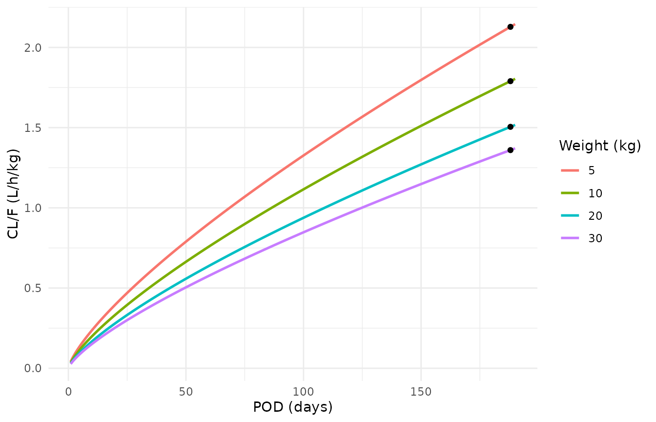

Replicates Figure 3 of Chen 2020: typical CL/F per kg against days post-transplant.

A 1% error in the clearance coefficient must break the tight identity:

stopifnot(all(abs(sim_grid$cl / (1.01 * published_cl(sim_grid$WT, sim_grid$POD)) - 1) > 1e-3))

Scale of the variability terms

Table II prints omega and sigma without saying whether they are standard deviations or variances, and the paper quotes no CV%. For V/F the question is moot (0.998 as an SD or as a variance gives SDs of 0.998 and 0.999). It matters for CL/F (SD 0.627 vs 0.792) and for the residual error (0.447 vs 0.669 proportional; 70.1 vs 8.4 ng/mL additive).

The prediction-corrected VPC (Chen 2020 Figure 2) settles it. At steady state a trough is proportional to 1/CL, so after prediction correction the spread is carried by the CL/F eta and the residual error. The figure’s median trough is about 170 ng/mL and the simulated 97.5th-percentile band runs from about 330 to 700 ng/mL in the early bins and about 150 to 550 ng/mL in the last bin. The 97.5th percentile of Y = F (1 + eps1) + eps2 with F = 170 exp(eta_CL) is computed deterministically on a grid below.

pct975 <- function(om_cl, s_prop, s_add, f_typ = 170) {
  node <- seq(-6, 6, length.out = 241)
  w <- dnorm(node) / sum(dnorm(node))
  f <- f_typ * exp(om_cl * node)
  # Y | F is normal with SD sqrt((F * s_prop)^2 + s_add^2).
  sd_y <- sqrt((f * s_prop)^2 + s_add^2)
  p_above <- function(y) sum(w * pnorm(y, f, sd_y, lower.tail = FALSE))
  uniroot(function(y) p_above(y) - 0.025, c(f_typ, 50 * f_typ))$root
}
scale_tab <- tibble::tibble(
  reading = c("SD (as encoded)", "variance"),
  om_cl = c(0.627, sqrt(0.627)),
  s_prop = c(0.447, sqrt(0.447)),
  s_add = c(70.071, sqrt(70.071))
) |>
  dplyr::rowwise() |>
  dplyr::mutate(p975 = pct975(om_cl, s_prop, s_add)) |>
  dplyr::ungroup()

stopifnot(
  # The SD reading lands at the top of the published band ...
  scale_tab$p975[1] < 720,
  # ... and the variance reading sits far above anything in Figure 2.
  scale_tab$p975[2] > 900
)
scale_tab |>
  dplyr::rename(
    "Reading" = reading, "SD of eta CL/F" = om_cl,
    "Proportional SD" = s_prop, "Additive SD (ng/mL)" = s_add,
    "97.5th percentile at 170 ng/mL" = p975
  ) |>
  knitr::kable(digits = 3, caption = "97.5th percentile implied by each reading of Table II, against the Figure 2 simulated band (about 150-700 ng/mL).")

97.5th percentile implied by each reading of Table II, against the Figure 2 simulated band (about 150-700 ng/mL).
Reading	SD of eta CL/F	Proportional SD	Additive SD (ng/mL)	97.5th percentile at 170 ng/mL
SD (as encoded)	0.627	0.447	70.071	697.309
variance	0.792	0.669	8.371	1016.272

The variance reading puts the 97.5th percentile near 1000 ng/mL, outside every bin of Figure 2; the SD reading is at the top of the band. The same authors’ Wang 2019 cyclosporin paper in the same journal prints omega on the SD scale, confirmed there by the CV%s quoted in its abstract. The model therefore takes the printed values as SDs.

Replicating the dose-finding simulation (Table III and Figure 4)

Chen 2020 simulated 1000 virtual children at each of 5, 10, 20 and 30 kg on 2 to 8 mg/kg/day split into two doses and reported the trough median with a 15th-85th percentile interval (Table III) and the probability of a trough between 50 and 350 ng/mL (Figure 4). The paper states neither the POD nor the sampling day used. Two features of Table III pin them down. First, the troughs barely depend on body weight: with CL/F scaling as WT^0.75 and dose as WT, a steady-state trough would rise by about 57% from 5 to 30 kg, yet Table III shows under 1%. The troughs must be early, while concentration is still close to accumulated dose / V/F, which scales out with weight. Second, the median at 1 mg/kg per dose is about four doses’ worth of 1 mg/kg / 93.6 L/kg. The reconstruction below therefore takes an initial-dose scenario at POD = 1 and the trough just before the fifth dose (48 h), without residual error. These choices are the maintainers’, and they are back-solved from the table.

The model is linear in dose, so one solve at 1 mg/kg per dose is scaled to each regimen. The IIV integral is computed on a fixed grid of eta values (no random cohort), passed to the typical-value model as per-subject lcl / lvc.

# The early troughs are driven mainly by V/F, so its axis gets the finer
# grid; the probability-of-target is an indicator integral and a coarse grid
# makes it step-shaped.
node_cl <- seq(-4.5, 4.5, length.out = 41)
node_v <- seq(-5, 5, length.out = 201)
w_cl <- dnorm(node_cl) / sum(dnorm(node_cl))
w_v <- dnorm(node_v) / sum(dnorm(node_v))
eta_grid <- tidyr::expand_grid(i_cl = seq_along(node_cl), i_v = seq_along(node_v)) |>
  dplyr::mutate(w = w_cl[i_cl] * w_v[i_v])

wquantile <- function(x, w, p) {
  o <- order(x)
  cw <- cumsum(w[o]) / sum(w)
  vapply(p, function(pp) x[o][which(cw >= pp)[1]], numeric(1))
}

trough_one_weight <- function(wt) {
  params <- eta_grid |>
    dplyr::mutate(
      id = dplyr::row_number(),
      lcl = log(29.2) + 0.627 * node_cl[i_cl],
      lvc = log(6550) + 0.998 * node_v[i_v]
    )
  ev <- dplyr::bind_rows(lapply(params$id, function(i) {
    tibble::tibble(
      id = i, time = c(0, 12, 24, 36, 48), evid = c(1L, 1L, 1L, 1L, 0L),
      amt = c(rep(wt, 4), NA_real_), cmt = c(rep("depot", 4), "central"),
      WT = wt, POD = 1
    )
  }))
  # rxode2 warns that a multi-subject solve has no omega; that is intended
  # here, as the between-subject spread is supplied by the eta grid.
  sim <- suppressWarnings(rxode2::rxSolve(
    mod_typical,
    events = ev,
    params = dplyr::select(params, id, lcl, lvc)
  )) |>
    as.data.frame() |>
    dplyr::filter(time == 48)
  tibble::tibble(WT = wt, Cc = sim$Cc, w = params$w[match(sim$id, params$id)])
}

troughs <- dplyr::bind_rows(lapply(c(5, 10, 20, 30), trough_one_weight))
#> ℹ omega/sigma items treated as zero: 'etalcl', 'etalvc'
#> ℹ omega/sigma items treated as zero: 'etalcl', 'etalvc'
#> ℹ omega/sigma items treated as zero: 'etalcl', 'etalvc'
#> ℹ omega/sigma items treated as zero: 'etalcl', 'etalvc'
stopifnot(nrow(troughs) == 4L * nrow(eta_grid))

regimens <- c(2, 3, 4, 5, 6, 7, 8)
sim_tab <- tidyr::expand_grid(WT = c(5, 10, 20, 30), mgkgday = regimens) |>
  dplyr::rowwise() |>
  dplyr::mutate(
    q = list(wquantile(
      troughs$Cc[troughs$WT == WT] * mgkgday / 2,
      troughs$w[troughs$WT == WT],
      c(0.15, 0.5, 0.85)
    )),
    q15 = q[1], med = q[2], q85 = q[3],
    pta = 100 * {
      cc <- troughs$Cc[troughs$WT == WT] * mgkgday / 2
      ww <- troughs$w[troughs$WT == WT]
      sum(ww[cc >= 50 & cc <= 350]) / sum(ww)
    }
  ) |>
  dplyr::ungroup() |>
  dplyr::select(-q)

# Chen 2020 Table III (median, 15th, 85th percentile), 5 and 30 kg columns.
# The 2 mg/kg/day 5 kg median is printed as 41.5; every other entry in the
# column is exactly proportional to dose with a 41.15 base, so 41.5 is taken
# as a transposition of 41.15.
tab3 <- tibble::tribble(
  ~WT, ~mgkgday, ~med_pub, ~q15_pub, ~q85_pub,
  5, 2, 41.15, 15.05, 104.81,
  5, 6, 123.45, 45.15, 314.43,
  30, 2, 41.54, 15.11, 108.09,
  30, 6, 124.62, 45.32, 324.29
)
# Chen 2020 Figure 4, read by the maintainers (probability, %, of a trough
# in 50-350 ng/mL); digitisation resolution about 0.3 percentage points.
fig4 <- tibble::tribble(
  ~mgkgday, ~WT5, ~WT10, ~WT20, ~WT30,
  2, 41.8, 42.0, 42.2, 42.3,
  3, 55.8, 56.1, 56.2, 56.1,
  4, 64.0, 63.6, 63.3, 62.8,
  5, 68.9, 68.4, 68.0, 67.9,
  6, 69.7, 68.8, 68.9, 68.9,
  7, 70.1, 69.7, 69.2, 69.1,
  8, 68.6, 67.9, 67.4, 67.0
) |>
  tidyr::pivot_longer(-mgkgday, names_to = "WT", values_to = "pta_pub") |>
  dplyr::mutate(WT = as.numeric(sub("WT", "", WT)))

tab3_check <- dplyr::inner_join(sim_tab, tab3, by = c("WT", "mgkgday")) |>
  dplyr::mutate(
    med_diff = 100 * (med / med_pub - 1),
    q15_diff = 100 * (q15 / q15_pub - 1),
    q85_diff = 100 * (q85 / q85_pub - 1)
  )
fig4_check <- dplyr::inner_join(sim_tab, fig4, by = c("WT", "mgkgday")) |>
  dplyr::mutate(pta_diff = pta - pta_pub)

stopifnot(
  nrow(tab3_check) == 4L,
  nrow(fig4_check) == 28L,
  # The published percentiles come from 1000 simulated children, so they
  # carry about 5% Monte Carlo error (15th/85th) and 3% (median).
  all(abs(tab3_check$med_diff) < 6),
  all(abs(tab3_check$q15_diff) < 10),
  all(abs(tab3_check$q85_diff) < 12),
  # Figure 4: about 1.5 points of Monte Carlo error on each published value.
  abs(median(fig4_check$pta_diff)) < 2,
  max(abs(fig4_check$pta_diff)) < 5,
  # Weight invariance, the feature that fixes the scenario.
  max(sim_tab$med[sim_tab$mgkgday == 2]) / min(sim_tab$med[sim_tab$mgkgday == 2]) < 1.02
)

tab3_check |>
  dplyr::select(WT, mgkgday, med, med_pub, q15, q15_pub, q85, q85_pub) |>
  dplyr::rename(
    "WT (kg)" = WT, "Dose (mg/kg/day)" = mgkgday,
    "Median, model" = med, "Median, Table III" = med_pub,
    "15th, model" = q15, "15th, Table III" = q15_pub,
    "85th, model" = q85, "85th, Table III" = q85_pub
  ) |>
  knitr::kable(digits = 2, caption = "Replicates Table III of Chen 2020 (trough ng/mL, 48 h after the first dose at POD = 1).")

Replicates Table III of Chen 2020 (trough ng/mL, 48 h after the first dose at POD = 1).
WT (kg)	Dose (mg/kg/day)	Median, model	Median, Table III	15th, model	15th, Table III	85th, model	85th, Table III
5	2	42.20	41.15	14.95	15.05	114.47	104.81
5	6	126.60	123.45	44.84	45.15	343.40	314.43
30	2	42.40	41.54	14.96	15.11	117.00	108.09
30	6	127.19	124.62	44.88	45.32	351.00	324.29

ggplot(fig4_check, aes(WT, pta, colour = factor(mgkgday))) +
  geom_line() +
  geom_point(aes(y = pta_pub), shape = 1, size = 2) +
  labs(x = "Weight (kg)", y = "Probability of target attainment (%)", colour = "mg/kg/day") +
  theme_minimal()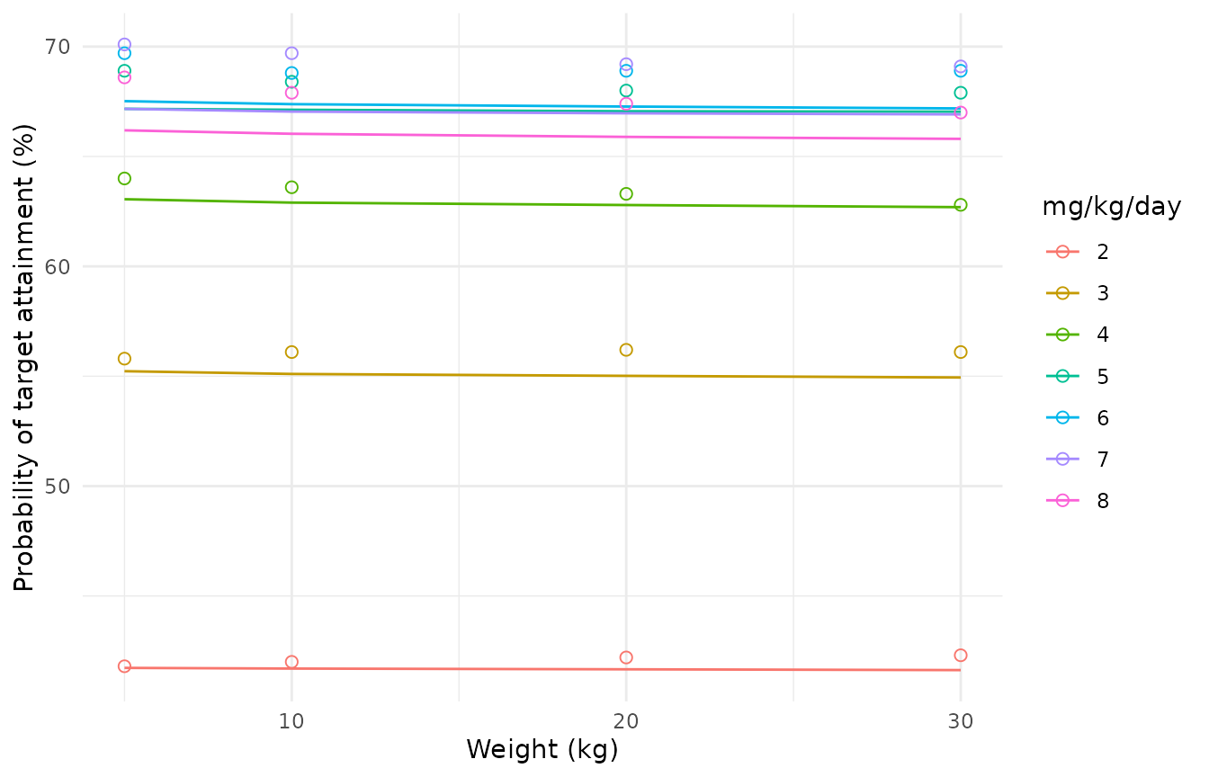

Replicates Figure 4 of Chen 2020: probability of a trough in 50-350 ng/mL. Lines, this model; points, values read from Figure 4.

The model reproduces the paper’s conclusion: 6 and 7 mg/kg/day give the highest probability of a 50-350 ng/mL trough, and at 7 mg/kg/day the 85th percentile exceeds 350 ng/mL at every weight (401, 404, 408, 410 ng/mL for 5, 10, 20 and 30 kg), which is why 6 mg/kg/day was chosen.

Steady-state PKNCA check

At a fixed POD the model is linear and time-invariant, so at steady state AUC_tau = Dose / (CL/F) exactly. The typical 7.6 kg child (cohort median) at POD 51.5 days receives 6 mg/kg/day as 22.8 mg every 12 h for 60 days; PKNCA is run on the final dosing interval for each of the four simulated weights.

wts <- c(5, 7.6, 20, 30)
tau <- 12
n_dose <- 120
t_last <- (n_dose - 1) * tau
obs_t <- t_last + seq(0, tau, by = 0.25)
ev_ss <- dplyr::bind_rows(lapply(seq_along(wts), function(i) {
  dplyr::bind_rows(
    tibble::tibble(id = i, time = (0:(n_dose - 1)) * tau, evid = 1L,
                   amt = 3 * wts[i], cmt = "depot"),
    tibble::tibble(id = i, time = obs_t, evid = 0L, amt = NA_real_, cmt = "central")
  ) |>
    dplyr::mutate(WT = wts[i], POD = 51.5, treatment = paste0(wts[i], " kg"))
})) |>
  dplyr::arrange(id, time, dplyr::desc(evid))

sim_ss <- rxode2::rxSolve(mod_typical, events = ev_ss, keep = c("WT", "treatment")) |>
  as.data.frame()
#> ℹ omega/sigma items treated as zero: 'etalcl', 'etalvc'
#> Warning: multi-subject simulation without without 'omega'

conc_ss <- sim_ss |>
  dplyr::filter(!is.na(Cc)) |>
  dplyr::mutate(time = time - t_last) |>
  dplyr::select(id, treatment, time, Cc)
dose_ss <- ev_ss |>
  dplyr::filter(evid == 1, time == t_last) |>
  dplyr::mutate(time = 0) |>
  dplyr::select(id, treatment, time, amt)

nca_ss <- PKNCA::pk.nca(PKNCA::PKNCAdata(
  PKNCA::PKNCAconc(conc_ss, Cc ~ time | treatment + id, concu = "ng/mL", timeu = "h"),
  PKNCA::PKNCAdose(dose_ss, amt ~ time | treatment + id, doseu = "mg"),
  intervals = data.frame(start = 0, end = tau, auclast = TRUE, cmax = TRUE, cmin = TRUE)
))
nca_ss_wide <- as.data.frame(nca_ss$result) |>
  dplyr::select(treatment, PPTESTCD, PPORRES) |>
  tidyr::pivot_wider(names_from = PPTESTCD, values_from = PPORRES) |>
  dplyr::mutate(
    WT = as.numeric(sub(" kg", "", treatment)),
    auc_expected = 3 * WT / published_cl(WT, 51.5) * 1000,
    pct_diff = 100 * (auclast / auc_expected - 1)
  )

# Deterministic solve against its own closed form: a tight bound is correct.
stopifnot(nrow(nca_ss_wide) == 4L, all(abs(nca_ss_wide$pct_diff) < 0.5))

nca_ss_wide |>
  dplyr::arrange(WT) |>
  dplyr::select(treatment, cmax, cmin, auclast, auc_expected, pct_diff) |>
  dplyr::rename(
    "Weight" = treatment, "Cmax (ng/mL)" = cmax, "Cmin (ng/mL)" = cmin,
    "AUC0-12 PKNCA (ng*h/mL)" = auclast, "Dose/(CL/F) (ng*h/mL)" = auc_expected,
    "Difference (%)" = pct_diff
  ) |>
  knitr::kable(digits = 2, caption = "Typical-value steady state at 6 mg/kg/day and POD 51.5 days.")

Typical-value steady state at 6 mg/kg/day and POD 51.5 days.
Weight	Cmax (ng/mL)	Cmin (ng/mL)	AUC0-12 PKNCA (ng*h/mL)	Dose/(CL/F) (ng*h/mL)	Difference (%)
5 kg	317.66	297.84	3717.83	3717.96	0.00
7.6 kg	351.85	332.02	4128.07	4128.24	0.00
20 kg	445.91	426.07	5257.06	5257.99	-0.02
30 kg	492.55	472.70	5816.70	5818.92	-0.04

Chen 2020 reports no NCA parameters, so there is no published NCA table to compare against.

Stochastic trough profile with time-varying POD

A cohort of 200 children at the median weight (7.6 kg) starts 6 mg/kg/day on POD 1, with POD advancing with the simulation clock, and troughs are recorded daily for 60 days (residual error included).

rxode2::rxSetSeed(20200601)
n_sub <- 200
days <- 60
dose_t <- seq(0, days * 24 - tau, by = tau)
obs_d <- seq(24, days * 24, by = 24) - 1e-6
ev_vpc <- dplyr::bind_rows(
  tidyr::expand_grid(id = seq_len(n_sub), time = dose_t) |>
    dplyr::mutate(evid = 1L, amt = 3 * 7.6, cmt = "depot"),
  tidyr::expand_grid(id = seq_len(n_sub), time = obs_d) |>
    dplyr::mutate(evid = 0L, amt = NA_real_, cmt = "central")
) |>
  dplyr::mutate(WT = 7.6, POD = 1 + time / 24) |>
  dplyr::arrange(id, time, dplyr::desc(evid))

sim_vpc <- rxode2::rxSolve(mod, events = ev_vpc, keep = "POD") |>
  as.data.frame()
vpc_sum <- sim_vpc |>
  dplyr::filter(!is.na(sim)) |>
  dplyr::mutate(day = round(time / 24)) |>
  dplyr::group_by(day) |>
  dplyr::summarise(
    q15 = quantile(sim, 0.15), med = median(sim), q85 = quantile(sim, 0.85),
    .groups = "drop"
  )
ggplot(vpc_sum, aes(day, med)) +
  annotate("rect", xmin = -Inf, xmax = Inf, ymin = 50, ymax = 350, alpha = 0.1, fill = "darkgreen") +
  geom_ribbon(aes(ymin = q15, ymax = q85), alpha = 0.3) +
  geom_line(linewidth = 0.9) +
  labs(x = "Day of therapy", y = "Ciclosporin trough (ng/mL)") +
  theme_minimal()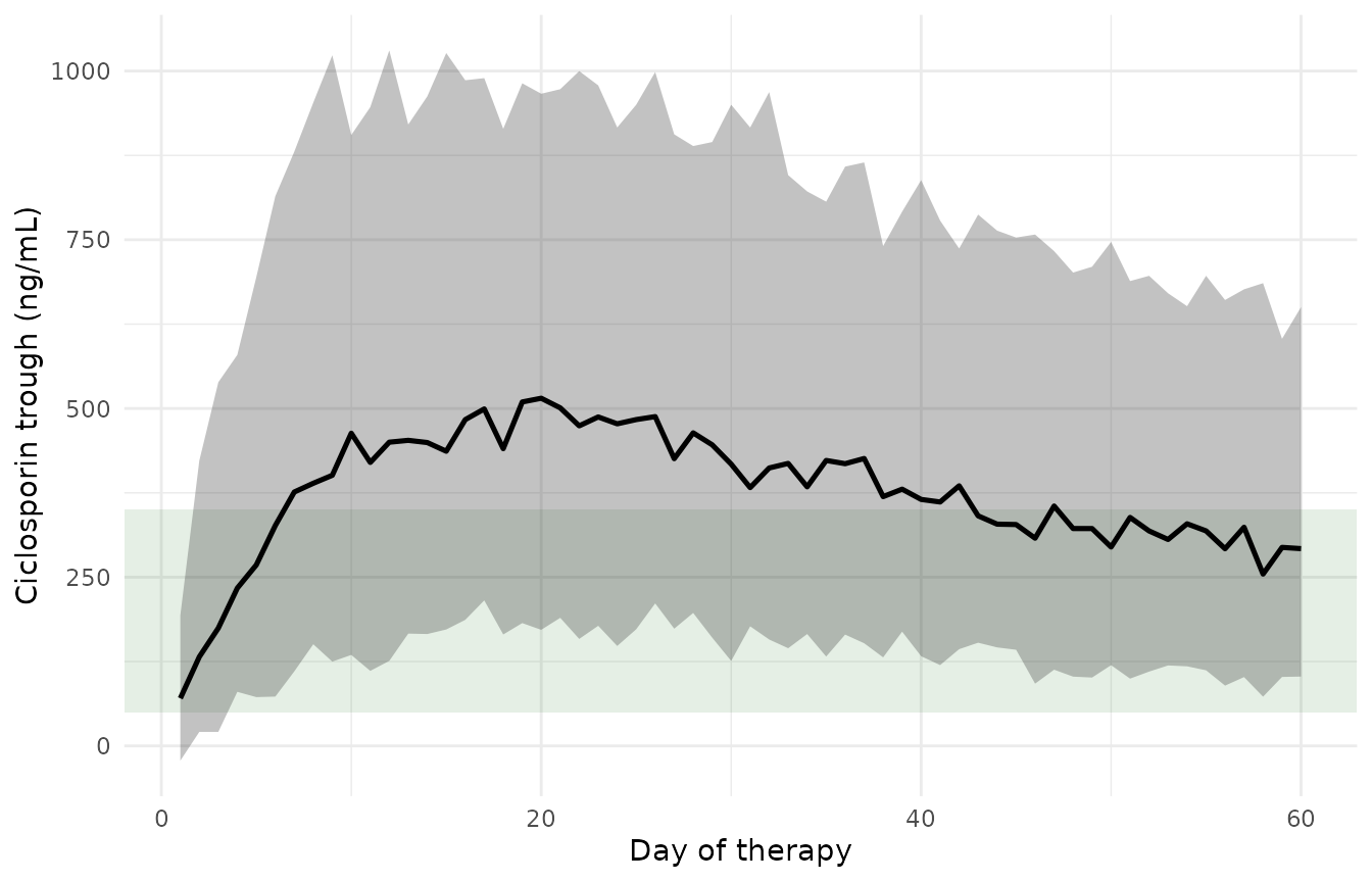

Simulated troughs (median and 15th-85th percentile) at 6 mg/kg/day from POD 1; the shaded band is the 50-350 ng/mL target.

Because clearance is near zero immediately after transplant and rises with POD, troughs accumulate over the first weeks and then fall as clearance catches up. The paper’s dose recommendation concerns the initial dose only; it was not designed for, and should not be read as, a maintenance regimen.

Assumptions and deviations

Omega and sigma scale. Table II does not name its scale. The values are read as standard deviations, on the evidence of the pcVPC (above) and the same group’s convention in Wang 2019. For V/F the two readings are indistinguishable.
Table III / Figure 4 scenario. The paper does not state the POD or sampling time of its dose-finding simulation. POD = 1 with the trough 48 h after the first of twice-daily doses, without residual error, was back-solved from the weight invariance and dose scaling of Table III, and it reproduces Figure 4. No model parameter was adjusted.
Table III typo. The 5 kg, 2 mg/kg/day median is printed as 41.5 ng/mL; the rest of the column is exactly dose-proportional to 41.15, which is used here.
POD at zero. The power form makes CL/F zero at POD = 0. The observed data start at POD = 1; supply POD >= 1.
Covariates without canonical columns. Mycophenolate mofetil and tacrolimus co-medication, mean corpuscular hemoglobin and mean corpuscular hemoglobin concentration were screened but have no canonical column; they are recorded in the model’s population notes only.
Figure readings. Figure 3 and Figure 4 values were read by the maintainers from the published figures.