Capivasertib (Fernandez-Teruel 2024)
Source:vignettes/articles/FernandezTeruel_2024_capivasertib.Rmd
FernandezTeruel_2024_capivasertib.RmdModel and source
#> ℹ parameter labels from comments will be replaced by 'label()'- Citation: Fernandez-Teruel C, Cullberg M, Eberlein C, Barry ST, Zhou D. Population Pharmacokinetics of Capivasertib in Patients with Advanced or Metastatic Solid Tumours. Clin Pharmacokinet. 2024;63(8):1191-1204. doi:10.1007/s40262-024-01407-x.
- Description: Three-compartment population PK model for capivasertib (oral pan-AKT inhibitor) with parallel first-order and zero-order absorption, absorption lag time, and sigmoidal time-dependent auto-inhibition of apparent clearance, in patients with advanced or metastatic solid tumours (Fernandez-Teruel 2024)
- Article: https://doi.org/10.1007/s40262-024-01407-x
Capivasertib is a first-in-class, selective inhibitor of all three AKT isoforms. Fernandez-Teruel 2024 pooled the plasma pharmacokinetic data from four phase I and II studies in patients with advanced or metastatic solid tumours and fitted a single population PK model in NONMEM 7.3.0 with PsN 4.4.8.
Population
| Field | Value |
|---|---|
| species | human |
| n_subjects | 441 |
| n_studies | 4 |
| n_observations | 3963 |
| age_range | 27-87 years |
| age_median | 56 years |
| weight_range | 32-129 kg |
| weight_median | 67 kg |
| sex_female_pct | 79.6 |
| race_ethnicity | White 74.1; Black 2; Asian 17; American Indian or Alaska Native 2.9; Other 2.9; Missing 0.9 |
| disease_state | Advanced or metastatic solid tumours (including advanced / metastatic breast cancer) |
| dose_range | 80-800 mg orally twice daily over 21-day and 28-day cycles, as monotherapy or with paclitaxel or fulvestrant; continuous dosing or one of two intermittent schedules, 4 days on / 3 days off (4/3, 73.7% of patients) or 2 days on / 5 days off (2/5, 10.9%) |
| renal_function | Normal (CrCL >= 90 mL/min) 58.0%, mild (60-89) 32.9%, moderate (30-59) 8.8%, no severe impairment |
| hepatic_function | Normal 67.1%, mild 31.3%, moderate 1.4%, no severe impairment |
| co_medication | Paclitaxel 20.4% (BEECH only), fulvestrant 16.8% (Study 1 only), acid-reducing agent 31.5% |
| regions | Global (Study 1, BEECH and OAK multinational; Study 4 all-Japanese) |
| notes | Pooled from four phase I / II studies: Study 1 (n = 280), BEECH (n = 90), Study 4 (n = 41, Japanese) and OAK (n = 30). Baseline demographics are Fernandez-Teruel 2024 Table 2 (key covariates) and ESM Table 2 (other covariates). 559 of 4522 samples were excluded, 141 of them below the 1.00 ng/mL limit of quantification. |
The analysis dataset was 3963 plasma concentrations from 441 patients across Study 1 (n = 280), BEECH (n = 90), Study 4 (n = 41, all Japanese) and OAK (n = 30). Baseline demographics are Fernandez-Teruel 2024 Table 2: median age 56 years (range 27-87), median body weight 67 kg (range 32-129), median creatinine clearance 97 mL/min (range 35-304), 79.6% female, 74.1% white. Capivasertib was given orally at 80-800 mg twice daily, as monotherapy or with paclitaxel or fulvestrant, on a continuous schedule (15.4% of patients) or one of two intermittent schedules, 4 days on / 3 days off (4/3, 73.7%) or 2 days on / 5 days off (2/5, 10.9%).
Model structure
Fernandez-Teruel 2024 Fig. 2 shows a three-compartment disposition model fed by two parallel absorption routes from a single oral dose:
- a fraction
F1enters a first-orderdepotwith rate constantKaand lag timeALAG1; - the remaining
1 - F1is delivered as a zero-order input straight into thecentralcompartment over a durationD2.
Apparent clearance is time-dependent: capivasertib is both a CYP3A4
substrate and a weak time-dependent CYP3A4 inhibitor, and
CL/F falls from its initial value along a sigmoid in time.
The paper’s covariate equations, transcribed verbatim from Sect. 3.3,
are
| Equation | |
|---|---|
| (a) | F1_i = exp(LogitF1 * (BBW/67)^F1_BBW + eta) / (1 + exp(LogitF1 * (BBW/67)^F1_BBW + eta)) |
| (b) | F2_i = 1 - F1_i |
| (c) | ALAG1_i = (Lag1_tab * (1 - CAP) + Lag1_cap * CAP) * (1 - FASTED) * exp(eta) |
| (d) | CL0/F_i = CL0/F * (1 + (BBW - 67) * CL0_BBW) * exp(eta) |
| (e) | CL/F_i = CL0/F_i * (1 - exp(Imax_i) * Time^5 / (T50^5 + Time^5)) |
| (f) | Imax_i = Imax * (1 + (DOSE - 480) * Imax_dose) * (1 + PACL * Imax_pacl) * exp(eta) |
Two features of this parameterisation are worth flagging because they are easy to mis-transcribe.
-
Imaxis a log. Table 3 reportsImax = -1.54, and equation (e) puts it inside an exponential, so the maximal fractional inhibition ofCL/Fisexp(-1.54) = 0.214. Reading-1.54as the fraction itself would make clearance rise by 154%. The model file therefore stores it aslcl_time_max <- -1.54on the registered log scale and applies the sign inmodel(), exactly asMasters_2022_avelumab.Rdoes for the same sigmoidal-in-time clearance family. Section Time-dependent clearance below shows this reading is the one that reproduces the paper’s own 18% / 22% / 54% reductions. -
The covariate and random effects on
Imaxare multiplicative on the log scale, not on the fraction. BecauseImax < 0, the multiplier acts in the counter-intuitive direction: a multiplier above 1 drivesImax_ifurther negative, shrinksexp(Imax_i), and therefore shallows the auto-inhibition and raisesCL/F; a multiplier below 1 deepens it. The negative dose slope (Imax_dose = -0.00183) makes the multiplier shrink as dose rises (1.146 at 400 mg, 1 at 480 mg, 0.414 at 800 mg), so the inhibition still grows with dose – which is what produces the more-than-dose-proportional exposure above 480 mg.
Every disposition, absorption and clearance parameter is apparent
(/F): the pooled dataset has no intravenous arm, so
F is not identifiable and is absorbed into CL,
V and Q.
Source trace
Every ini() entry in
inst/modeldb/specificDrugs/FernandezTeruel_2024_capivasertib.R
carries an in-file comment naming its source. They are collected here
for review.
| Model parameter | Paper symbol | Value | Source location |
|---|---|---|---|
lka |
Ka | 0.417 1/h | Table 3 |
lcl |
CL0/F | 62.2 L/h | Table 3 |
lvc |
V2/F | 47.9 L | Table 3 |
lvp |
V3/F | 113 L | Table 3 |
lq |
Q3/F | 2.66 L/h | Table 3 |
lvp2 |
V4/F | 94.7 L | Table 3 |
lq2 |
Q4/F | 21.8 L/h | Table 3 |
ld1 |
D2 | 45.1 h | Table 3 |
logitffo |
Logit F1 | 1.4 | Table 3; equation (a) |
ltlag_tab |
Lag1_tab | 0.212 h | Table 3; equation (c) |
ltlag_cap |
Lag1_cap | 0.46 h | Table 3; equation (c) |
lcl_time_max |
Imax | -1.54 (log scale) | Table 3; equation (e) |
lcl_t50 |
T50 | 67.4 h | Table 3; equation (e) |
lcl_time_hill |
Hill | 5 (fixed) | Sect. 3.2 (“a Hill parameter fixed at five”); equation (e) |
e_wt_cl |
CL0_BBW | 0.00585 /kg | Table 3; equation (d) |
e_wt_logitffo |
F1_BBW | -1.11 | Table 3; equation (a) |
e_dose_cl_time_max |
Imax_dose | -0.00183 /mg | Table 3; equation (f) |
e_pacl_cl_time_max |
Imax_pacl | 1.15 | Table 3; equation (f) |
etalcl |
CL0/F BSV | 39.3% CV | Table 3 |
etalvc |
V2/F BSV | 114% CV | Table 3 |
etalcl_time_max |
Imax BSV | 70.6% CV | Table 3 |
etaltlag |
Lag1 BSV | 63% CV | Table 3 |
etalogitffo |
Logit F1 BSV | 96.2% CV | Table 3; additive on the logit scale per Sect. 3.2 |
etalka, etald1
|
Ka, D2 BSV | 15% CV (fixed) | Table 3 footnote |
propSd |
RUV proportional | 43.9% CV | Table 3 |
addSd |
RUV additive | 0.504 ug/L | Table 3 |
| Structural equations (a)-(f) | n/a | n/a | Sect. 3.3, displayed equations |
| Three-compartment layout, parallel absorption | n/a | n/a | Fig. 2 and Sect. 3.2 |
Verification helpers
mod <- readModelDb("FernandezTeruel_2024_capivasertib")
tv  <- rxode2::zeroRe(mod)   # typical-value (all etas set to zero) version
#> ℹ parameter labels from comments will be replaced by 'label()'

# Dosing-time grids for the three schedules the paper simulated. All are
# twice-daily (q12h) within a dosing day; the schedules differ in which days
# of each 7-day week carry doses.
dose_times <- function(schedule, n_weeks) {
  days <- switch(
    schedule,
    "continuous" = seq_len(n_weeks * 7L) - 1L,
    "4/3"        = unlist(lapply(seq_len(n_weeks) - 1L, function(w) w * 7L + 0:3)),
    "2/5"        = unlist(lapply(seq_len(n_weeks) - 1L, function(w) w * 7L + 0:1))
  )
  sort(c(days * 24, days * 24 + 12))
}

# Build an event table. Each administration is TWO dose records carrying the
# same amt: one into `depot` (scaled by f(depot) = ffo, lagged by alag(depot))
# and one into `central` (scaled by f(central) = 1 - ffo, delivered as a
# zero-order input whose duration is modelled, hence rate = -2).
make_events <- function(ids, dose, dosing_times, obs_times, WT = 67,
                        FORM_CAPSULE = 0, FASTED_STRICT = 0,
                        CONMED_PACLITAXEL = 0, treatment = "") {
  subj <- data.frame(id = ids, WT = WT)
  dos <- merge(subj, data.frame(time = dosing_times))
  dos <- rbind(
    transform(dos, amt = dose, evid = 1L, cmt = "depot",   rate = 0),
    transform(dos, amt = dose, evid = 1L, cmt = "central", rate = -2)
  )
  obs <- transform(merge(subj, data.frame(time = obs_times)),
                   amt = NA_real_, evid = 0L, cmt = "central", rate = 0)
  ev <- rbind(dos, obs)
  ev$FORM_CAPSULE <- FORM_CAPSULE
  ev$FASTED_STRICT <- FASTED_STRICT
  ev$CONMED_PACLITAXEL <- CONMED_PACLITAXEL
  ev$DOSE_CAPIVASERTIB_MG <- dose
  ev$treatment <- treatment
  ev[order(ev$id, ev$time, -ev$evid), ]
}

# Linear-trapezoidal AUC of Cc over [a, b] for a single-subject solve.
auc_window <- function(sim, a, b) {
  d <- sim[sim$time >= a & sim$time <= b, ]
  d <- d[order(d$time), ]
  sum(diff(d$time) * (head(d$Cc, -1) + tail(d$Cc, -1)) / 2)
}

# Week-3, 4th-dosing-day interval of the (4/3) schedule. The paper predicts
# steady state "on every third and fourth dosing day each week from the second
# week" (Sect. 3.2), so this 12 h window is where AUC12,ss and Cmax,ss live.
ss_start <- 17 * 24
ss_end   <- ss_start + 12

# Solve the typical-value model over the first dosing interval plus the
# steady-state interval and return the quantities the paper reports.
tv_profile <- function(dose = 400, WT = 67, FORM_CAPSULE = 0,
                       FASTED_STRICT = 0, CONMED_PACLITAXEL = 0) {
  obs <- sort(unique(c(seq(0, 12, by = 0.02), seq(ss_start, ss_end, by = 0.02))))
  ev <- make_events(1L, dose, dose_times("4/3", 3L), obs, WT = WT,
                    FORM_CAPSULE = FORM_CAPSULE, FASTED_STRICT = FASTED_STRICT,
                    CONMED_PACLITAXEL = CONMED_PACLITAXEL)
  s <- as.data.frame(rxode2::rxSolve(tv, ev, addDosing = FALSE))
  ss <- s[s$time >= ss_start, ]
  fd <- s[s$time <= 12, ]
  list(
    auc12_ss   = auc_window(s, ss_start, ss_end),
    cmax_ss    = max(ss$Cc),
    tmax_ss    = ss$time[which.max(ss$Cc)] - ss_start,
    auc12_dose1 = auc_window(s, 0, 12),
    tmax_dose1 = fd$time[which.max(fd$Cc)]
  )
}

# Collect claim / published / reproduced rows so the gate and the rendered
# table are driven by exactly the same numbers. `acc` is an environment
# (reference semantics) so `claim()` can append without superassignment.
acc <- new.env(parent = emptyenv())
acc$rows <- list()
claim <- function(what, published, reproduced, tolerance, unit = "",
                  deviation = FALSE) {
  acc$rows[[length(acc$rows) + 1L]] <- tibble::tibble(
    Quantity = what, Unit = unit, Published = published,
    Reproduced = reproduced, Tolerance = tolerance,
    Pass = abs(reproduced - published) <= tolerance, Deviation = deviation
  )
  invisible(reproduced)
}
Internal identities
These checks are deterministic functions of the ini()
values – no simulated cohort is involved – so they are gated tightly.
Each one is a quantity Fernandez-Teruel 2024 states in prose but did not
put in Table 3, which makes them independent tests of the transcription
rather than restatements of it.
p <- setNames(ui$theta, names(ui$theta))
Vss <- exp(p[["lvc"]]) + exp(p[["lvp"]]) + exp(p[["lvp2"]])
claim("Apparent volume of distribution at steady state (Vss = V2 + V3 + V4)",
      255.6, Vss, 0.2, "L")

# Fraction absorbed by the first-order route at the 67 kg reference weight.
ffo_ref <- 1 / (1 + exp(-p[["logitffo"]]))
claim("Fraction of the dose absorbed by the first-order route at 67 kg",
      0.80, ffo_ref, 0.01, "fraction")

# Disposition half-lives are the eigenvalues of the three-compartment matrix.
disposition_half_lives <- function(cl) {
  vc <- exp(p[["lvc"]]); vp <- exp(p[["lvp"]]); vp2 <- exp(p[["lvp2"]])
  q  <- exp(p[["lq"]]);  q2 <- exp(p[["lq2"]])
  kel <- cl / vc; k12 <- q / vc; k21 <- q / vp; k13 <- q2 / vc; k31 <- q2 / vp2
  A <- matrix(c(-(kel + k12 + k13), k21,  k31,
                 k12,              -k21,  0,
                 k13,               0,   -k31), nrow = 3, byrow = TRUE)
  sort(log(2) / -Re(eigen(A)$values))
}

# CL/F(t) for the typical patient, from equations (e) and (f).
clf_at <- function(time, dose = 400, WT = 67, CONMED_PACLITAXEL = 0) {
  imax_i <- p[["lcl_time_max"]] *
    (1 + (dose - 480) * p[["e_dose_cl_time_max"]]) *
    (1 + CONMED_PACLITAXEL * p[["e_pacl_cl_time_max"]])
  hill <- exp(p[["lcl_time_hill"]]); t50 <- exp(p[["lcl_t50"]])
  exp(p[["lcl"]]) * (1 + (WT - 67) * p[["e_wt_cl"]]) *
    (1 - exp(imax_i) * time^hill / (t50^hill + time^hill))
}

hl_first <- disposition_half_lives(exp(p[["lcl"]]))
hl_multi <- disposition_half_lives(clf_at(120))
for (i in seq_len(3)) {
  claim(sprintf("Disposition half-life t1/2-%s, first dose",
                c("alpha", "beta", "gamma")[i]),
        c(0.37, 4.2, 31)[i], hl_first[i], c(0.05, 0.2, 1.0)[i], "h")
  claim(sprintf("Disposition half-life t1/2-%s, multiple doses at 400 mg",
                c("alpha", "beta", "gamma")[i]),
        c(0.42, 4.4, 31)[i], hl_multi[i], c(0.05, 0.2, 1.0)[i], "h")
}
ref <- tv_profile()
#> ℹ omega/sigma items treated as zero: 'etalcl', 'etalvc', 'etalcl_time_max', 'etaltlag', 'etalogitffo', 'etalka', 'etald1'

claim("Tmax at steady state, 400 mg b.i.d. (4/3)", 1.4, ref$tmax_ss, 0.15, "h")
claim("AUC12,ss, 400 mg b.i.d. (4/3)", 7730, ref$auc12_ss, 300, "ug*h/L")
claim("Cmax,ss, 400 mg b.i.d. (4/3)", 1340, ref$cmax_ss, 70, "ug/L")

# Accumulation ratio: AUC over the steady-state interval divided by AUC over
# the first dosing interval.
r_acc <- ref$auc12_ss / ref$auc12_dose1
claim("Accumulation ratio, 400 mg b.i.d. (4/3)", 1.58, r_acc, 0.05, "ratio")

# Effective half-life implied by that accumulation ratio (Gidal 2017, the
# method Fernandez-Teruel 2024 cites as reference 22).
t_half_eff <- -12 * log(2) / log(1 - 1 / r_acc)
claim("Effective half-life, 400 mg b.i.d. (4/3)", 8.34, t_half_eff, 0.4, "h")
Time-dependent clearance (Fig. 4)
# Replicates Figure 4 of Fernandez-Teruel 2024: CL/F time course after
# twice-daily dosing, by dose level.
clf_grid <- tidyr::expand_grid(
  dose = c(400, 480, 800),
  time = seq(0, 336, by = 1)
) |>
  mutate(
    CLF = clf_at(time, dose = dose),
    treatment = factor(paste0(dose, " mg b.i.d."),
                       levels = paste0(c(400, 480, 800), " mg b.i.d."))
  )

ggplot(clf_grid, aes(time, CLF, colour = treatment)) +
  geom_line(linewidth = 0.8) +
  geom_vline(xintercept = 120, linetype = "dashed", colour = "grey40") +
  scale_x_continuous(breaks = seq(0, 336, by = 48)) +
  labs(x = "Time (h)", y = "CL/F (L/h)", colour = NULL,
       title = "Figure 4 - apparent clearance time course",
       caption = paste("Replicates Figure 4 of Fernandez-Teruel 2024.",
                       "Dashed line marks 120 h.")) +
  theme_bw() + theme(legend.position = "bottom")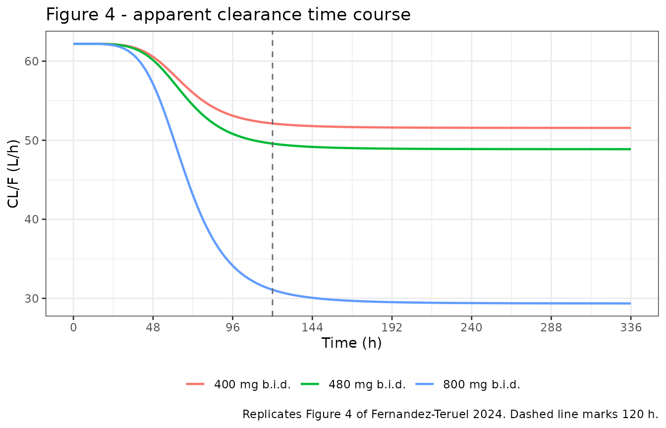
# Sect. 3.5: CL/F "decreased by 18%, 22% and 54% after approximately 120 h at
# 400, 480 and 800 mg".
cl_drop <- vapply(c(400, 480, 800),
                  function(d) 100 * (1 - clf_at(120, dose = d) / clf_at(0, dose = d)),
                  numeric(1))
cl_drop_inf <- vapply(c(400, 480, 800),
                      function(d) 100 * (1 - clf_at(1e6, dose = d) / clf_at(0, dose = d)),
                      numeric(1))
for (i in seq_len(3)) {
  claim(sprintf("Reduction in CL/F at 120 h, %s mg", c(400, 480, 800)[i]),
        c(18, 22, 54)[i], cl_drop[i], 4.5, "%", deviation = TRUE)
}

tibble::tibble(
  Dose = paste0(c(400, 480, 800), " mg"),
  `Published reduction at ~120 h (%)` = c(18, 22, 54),
  `Reproduced at 120 h (%)` = round(cl_drop, 1),
  `Reproduced asymptote (%)` = round(cl_drop_inf, 1)
) |>
  knitr::kable(caption = paste(
    "Auto-inhibition of CL/F. Reproduced values run about 1-2 percentage points",
"below the published ones; see Assumptions and deviations."))| Dose | Published reduction at ~120 h (%) | Reproduced at 120 h (%) | Reproduced asymptote (%) |
|---|---|---|---|
| 400 mg | 18 | 16.2 | 17.1 |
| 480 mg | 22 | 20.3 | 21.4 |
| 800 mg | 54 | 50.0 | 52.8 |
# Sect. 3.5 / ESM Fig. 3a: concomitant paclitaxel raises steady-state CL/F.
# The published ratios are compared against their own bootstrap intervals.
cl_ratio <- function(..., time = 120) clf_at(time, ...) / clf_at(time)
ratio_tab <- tibble::tibble(
  Covariate = c("Body weight 47 kg (5th percentile)",
                "Body weight 99 kg (95th percentile)",
                "Concomitant paclitaxel"),
  `Published CLss/F ratio` = c(0.88, 1.20, 1.20),
  `Published 95% CI` = c("0.80-0.94", "1.09-1.31", "1.12-1.29"),
  Reproduced = round(c(cl_ratio(WT = 47), cl_ratio(WT = 99),
                       cl_ratio(CONMED_PACLITAXEL = 1)), 3)
)
ratio_tab$`Inside CI` <- c(
  ratio_tab$Reproduced[1] >= 0.80 && ratio_tab$Reproduced[1] <= 0.94,
  ratio_tab$Reproduced[2] >= 1.09 && ratio_tab$Reproduced[2] <= 1.31,
  ratio_tab$Reproduced[3] >= 1.12 && ratio_tab$Reproduced[3] <= 1.29
)
knitr::kable(ratio_tab, caption = paste(
  "Steady-state CL/F covariate ratios against the 67 kg / 400 mg / no-paclitaxel",
"reference (Fernandez-Teruel 2024 Sect. 3.5 and ESM Fig. 3a)."))| Covariate | Published CLss/F ratio | Published 95% CI | Reproduced | Inside CI |
|---|---|---|---|---|
| Body weight 47 kg (5th percentile) | 0.88 | 0.80-0.94 | 0.883 | TRUE |
| Body weight 99 kg (95th percentile) | 1.20 | 1.09-1.31 | 1.187 | TRUE |
| Concomitant paclitaxel | 1.20 | 1.12-1.29 | 1.168 | TRUE |
Deterministic concentration-time profiles (Fig. 5)
# Replicates Figure 5 of Fernandez-Teruel 2024: deterministic profiles at
# different schedules and twice-daily dose levels.
profile_grid <- tidyr::expand_grid(
  schedule = c("continuous", "4/3", "2/5"),
  dose     = c(400, 800)
)
profiles <- do.call(rbind, Map(function(sch, d) {
  ev <- make_events(1L, d, dose_times(sch, 3L), seq(0, 21 * 24, by = 0.5),
                    treatment = paste0(d, " mg, ", sch))
  s <- as.data.frame(rxode2::rxSolve(tv, ev, addDosing = FALSE))
  data.frame(time = s$time, Cc = s$Cc, schedule = sch, dose = d)
}, profile_grid$schedule, profile_grid$dose))
#> ℹ omega/sigma items treated as zero: 'etalcl', 'etalvc', 'etalcl_time_max', 'etaltlag', 'etalogitffo', 'etalka', 'etald1'
#> ℹ omega/sigma items treated as zero: 'etalcl', 'etalvc', 'etalcl_time_max', 'etaltlag', 'etalogitffo', 'etalka', 'etald1'
#> ℹ omega/sigma items treated as zero: 'etalcl', 'etalvc', 'etalcl_time_max', 'etaltlag', 'etalogitffo', 'etalka', 'etald1'
#> ℹ omega/sigma items treated as zero: 'etalcl', 'etalvc', 'etalcl_time_max', 'etaltlag', 'etalogitffo', 'etalka', 'etald1'
#> ℹ omega/sigma items treated as zero: 'etalcl', 'etalvc', 'etalcl_time_max', 'etaltlag', 'etalogitffo', 'etalka', 'etald1'
#> ℹ omega/sigma items treated as zero: 'etalcl', 'etalvc', 'etalcl_time_max', 'etaltlag', 'etalogitffo', 'etalka', 'etald1'

profiles |>
  mutate(schedule = factor(schedule, levels = c("continuous", "4/3", "2/5")),
         dose = factor(paste0(dose, " mg b.i.d."))) |>
  ggplot(aes(time / 24, Cc, colour = dose)) +
  geom_line(linewidth = 0.5) +
  facet_wrap(~schedule, ncol = 1) +
  scale_x_continuous(breaks = 0:21) +
  scale_y_log10() +
  labs(x = "Time (days)", y = "Capivasertib concentration (ug/L)", colour = NULL,
       title = "Figure 5 - deterministic profiles by schedule and dose",
       caption = "Replicates Figure 5 of Fernandez-Teruel 2024.") +
  theme_bw() + theme(legend.position = "bottom")
#> Warning in scale_y_log10(): log-10 transformation introduced infinite values.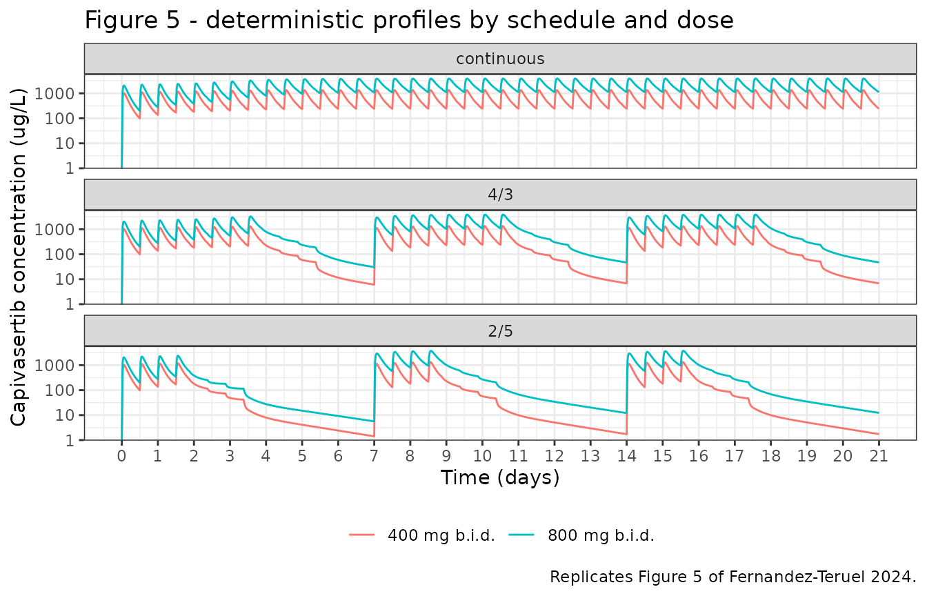
The (4/3) and (2/5) panels show the pattern the paper describes: exposure builds across the consecutive dosing days of each week, washes out during the days off, and the weekly envelope stabilises from the second week once the time-dependent clearance has settled (steady state “reached after approximately 120 h”, Sect. 3.5).
Formulation and food effects
# Sect. 4: food versus overnight fasted, and capsule versus tablet, "slightly
# delayed the time to maximum concentration at steady state without any impact
# on AUC12,ss or Cmax,ss". The reference is the tablet given semi-fasted.
variants <- tibble::tribble(
  ~label,                            ~FORM_CAPSULE, ~FASTED_STRICT,
  "Tablet, semi-fasted (reference)",  0,             0,
  "Tablet, overnight fasted",         0,             1,
  "Capsule, semi-fasted",             1,             0
)
variant_res <- do.call(rbind, Map(function(cap, fast) {
  r <- tv_profile(FORM_CAPSULE = cap, FASTED_STRICT = fast)
  data.frame(auc12_ss = r$auc12_ss, cmax_ss = r$cmax_ss, tmax_ss = r$tmax_ss)
}, variants$FORM_CAPSULE, variants$FASTED_STRICT))
#> ℹ omega/sigma items treated as zero: 'etalcl', 'etalvc', 'etalcl_time_max', 'etaltlag', 'etalogitffo', 'etalka', 'etald1'
#> ℹ omega/sigma items treated as zero: 'etalcl', 'etalvc', 'etalcl_time_max', 'etaltlag', 'etalogitffo', 'etalka', 'etald1'
#> ℹ omega/sigma items treated as zero: 'etalcl', 'etalvc', 'etalcl_time_max', 'etaltlag', 'etalogitffo', 'etalka', 'etald1'

form_tab <- tibble::tibble(
  Scenario = variants$label,
  `Tmax,ss (h)` = round(variant_res$tmax_ss, 3),
  `AUC12,ss ratio` = round(variant_res$auc12_ss / variant_res$auc12_ss[1], 4),
  `Cmax,ss ratio`  = round(variant_res$cmax_ss  / variant_res$cmax_ss[1], 4)
)
knitr::kable(form_tab, caption = paste(
  "Formulation and prandial state shift Tmax only, leaving AUC12,ss and Cmax,ss",
"unchanged (Fernandez-Teruel 2024 Sect. 4)."))| Scenario | Tmax,ss (h) | AUC12,ss ratio | Cmax,ss ratio |
|---|---|---|---|
| Tablet, semi-fasted (reference) | 1.40 | 1.0000 | 1.0000 |
| Tablet, overnight fasted | 1.20 | 1.0000 | 0.9993 |
| Capsule, semi-fasted | 1.66 | 0.9999 | 1.0006 |
# Exposure is unchanged to well within a percent; Tmax moves by the lag times.
stopifnot(
  max(abs(form_tab$`AUC12,ss ratio` - 1)) < 0.02,
  max(abs(form_tab$`Cmax,ss ratio`  - 1)) < 0.02,
  # Overnight fasting removes the whole lag (0.212 h for the tablet); the
  # capsule adds 0.46 - 0.212 = 0.248 h relative to the tablet reference.
  abs((form_tab$`Tmax,ss (h)`[1] - form_tab$`Tmax,ss (h)`[2]) - 0.212) < 0.05,
  abs((form_tab$`Tmax,ss (h)`[3] - form_tab$`Tmax,ss (h)`[1]) - 0.248) < 0.05
)
Covariate effects on exposure (Fig. 6)
# Replicates the covariate rows of Figure 6 of Fernandez-Teruel 2024: AUC12,ss
# and Cmax,ss relative to the reference subject (67 kg, 400 mg b.i.d. with
# tablets, semi-fasted, no paclitaxel).
cov_scenarios <- tibble::tribble(
  ~label,                  ~WT, ~CONMED_PACLITAXEL, ~pub_auc, ~pub_cmax,
  "Body weight 47 kg",      47,  0,                  1.14,     1.14,
  "Body weight 99 kg",      99,  0,                  NA,       NA,
  "Concomitant paclitaxel", 67,  1,                  0.84,     0.89
)
cov_res <- do.call(rbind, Map(function(w, pac) {
  r <- tv_profile(WT = w, CONMED_PACLITAXEL = pac)
  data.frame(auc = r$auc12_ss, cmax = r$cmax_ss)
}, cov_scenarios$WT, cov_scenarios$CONMED_PACLITAXEL))
#> ℹ omega/sigma items treated as zero: 'etalcl', 'etalvc', 'etalcl_time_max', 'etaltlag', 'etalogitffo', 'etalka', 'etald1'
#> ℹ omega/sigma items treated as zero: 'etalcl', 'etalvc', 'etalcl_time_max', 'etaltlag', 'etalogitffo', 'etalka', 'etald1'
#> ℹ omega/sigma items treated as zero: 'etalcl', 'etalvc', 'etalcl_time_max', 'etaltlag', 'etalogitffo', 'etalka', 'etald1'

cov_tab <- tibble::tibble(
  Covariate = cov_scenarios$label,
  `Published AUC12,ss ratio` = cov_scenarios$pub_auc,
  `Reproduced AUC12,ss ratio` = round(cov_res$auc / ref$auc12_ss, 3),
  `Published Cmax,ss ratio` = cov_scenarios$pub_cmax,
  `Reproduced Cmax,ss ratio` = round(cov_res$cmax / ref$cmax_ss, 3)
)
knitr::kable(cov_tab, caption = paste(
  "Exposure ratios against the reference subject, replicating the covariate",
  "rows of Fernandez-Teruel 2024 Figure 6. The 99 kg row is plotted but not",
"given a numeric ratio in the paper's text."))| Covariate | Published AUC12,ss ratio | Reproduced AUC12,ss ratio | Published Cmax,ss ratio | Reproduced Cmax,ss ratio |
|---|---|---|---|---|
| Body weight 47 kg | 1.14 | 1.132 | 1.14 | 1.142 |
| Body weight 99 kg | NA | 0.843 | NA | 0.839 |
| Concomitant paclitaxel | 0.84 | 0.849 | 0.89 | 0.898 |
for (i in which(!is.na(cov_scenarios$pub_auc))) {
  claim(sprintf("AUC12,ss ratio - %s", cov_scenarios$label[i]),
        cov_scenarios$pub_auc[i], cov_tab$`Reproduced AUC12,ss ratio`[i],
        0.03, "ratio")
  claim(sprintf("Cmax,ss ratio - %s", cov_scenarios$label[i]),
        cov_scenarios$pub_cmax[i], cov_tab$`Reproduced Cmax,ss ratio`[i],
        0.03, "ratio")
}
Dose proportionality
# Abstract and Sect. 3.5: AUC and Cmax "were proportional between the dose
# levels of 80-480 mg after multiple doses but more than proportional beyond
# 480 mg". Dose-normalised AUC12,ss, indexed to the 400 mg reference, makes the
# break visible.
dose_levels <- c(80, 160, 240, 320, 360, 400, 480, 560, 640, 800)
dose_res <- vapply(dose_levels, function(d) tv_profile(dose = d)$auc12_ss, numeric(1))
#> ℹ omega/sigma items treated as zero: 'etalcl', 'etalvc', 'etalcl_time_max', 'etaltlag', 'etalogitffo', 'etalka', 'etald1'
#> ℹ omega/sigma items treated as zero: 'etalcl', 'etalvc', 'etalcl_time_max', 'etaltlag', 'etalogitffo', 'etalka', 'etald1'
#> ℹ omega/sigma items treated as zero: 'etalcl', 'etalvc', 'etalcl_time_max', 'etaltlag', 'etalogitffo', 'etalka', 'etald1'
#> ℹ omega/sigma items treated as zero: 'etalcl', 'etalvc', 'etalcl_time_max', 'etaltlag', 'etalogitffo', 'etalka', 'etald1'
#> ℹ omega/sigma items treated as zero: 'etalcl', 'etalvc', 'etalcl_time_max', 'etaltlag', 'etalogitffo', 'etalka', 'etald1'
#> ℹ omega/sigma items treated as zero: 'etalcl', 'etalvc', 'etalcl_time_max', 'etaltlag', 'etalogitffo', 'etalka', 'etald1'
#> ℹ omega/sigma items treated as zero: 'etalcl', 'etalvc', 'etalcl_time_max', 'etaltlag', 'etalogitffo', 'etalka', 'etald1'
#> ℹ omega/sigma items treated as zero: 'etalcl', 'etalvc', 'etalcl_time_max', 'etaltlag', 'etalogitffo', 'etalka', 'etald1'
#> ℹ omega/sigma items treated as zero: 'etalcl', 'etalvc', 'etalcl_time_max', 'etaltlag', 'etalogitffo', 'etalka', 'etald1'
#> ℹ omega/sigma items treated as zero: 'etalcl', 'etalvc', 'etalcl_time_max', 'etaltlag', 'etalogitffo', 'etalka', 'etald1'
dn <- (dose_res / dose_levels) / (ref$auc12_ss / 400)

ggplot(tibble::tibble(dose = dose_levels, dn = dn), aes(dose, dn)) +
  geom_line() + geom_point() +
  geom_vline(xintercept = 480, linetype = "dashed", colour = "grey40") +
  labs(x = "Twice-daily dose (mg)",
       y = "Dose-normalised AUC12,ss (indexed to 400 mg)",
       title = "Dose proportionality of steady-state exposure",
       caption = paste("Dashed line at 480 mg, above which Fernandez-Teruel 2024",
                       "reports more-than-proportional exposure.")) +
  theme_bw()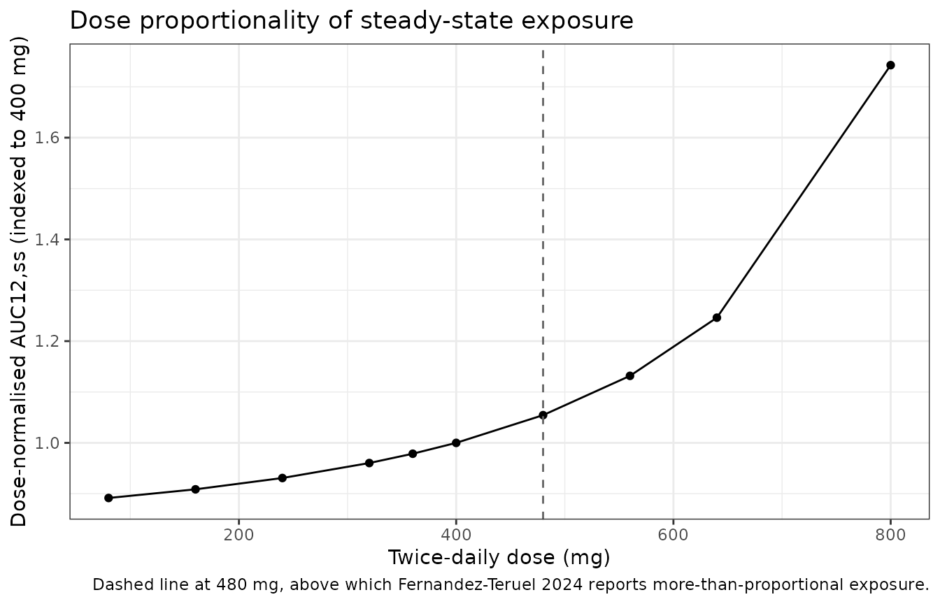
span_low  <- dn[dose_levels == 480] / dn[dose_levels == 80]
span_high <- dn[dose_levels == 800] / dn[dose_levels == 480]
# The claim is qualitative, so the gate is on the CONTRAST between the two
# ranges rather than on either one alone. Compare the rise in dose-normalised
# exposure PER MILLIGRAM, since the 80-480 mg range is wider than 480-800 mg:
# below 480 mg it is near-flat, above it the curve turns up sharply.
rate_low  <- (span_low  - 1) / (480 - 80)
rate_high <- (span_high - 1) / (800 - 480)
tibble::tibble(
  Range = c("80-480 mg", "480-800 mg"),
  `Rise in dose-normalised AUC12,ss` = round(c(span_low, span_high), 3),
  `Rise per mg` = signif(c(rate_low, rate_high), 3)
) |>
  knitr::kable(caption = paste(
    "Dose-normalised steady-state exposure is near-flat over the range",
    "Fernandez-Teruel 2024 calls dose-proportional and turns up sharply above",
"480 mg."))| Range | Rise in dose-normalised AUC12,ss | Rise per mg |
|---|---|---|
| 80-480 mg | 1.183 | 0.000456 |
| 480-800 mg | 1.652 | 0.002040 |
stopifnot(span_low < 1.3, span_high > 1.4, rate_high > 3 * rate_low)Virtual cohort
Original observed data are not publicly available. The cohort below is a virtual population whose body-weight distribution approximates the pooled trial demographics of Fernandez-Teruel 2024 Table 2 (median 67 kg, range 32-129 kg). All subjects receive the tablet formulation semi-fasted with no concomitant paclitaxel, matching the reference subject of the paper’s forest plots.
# set.seed() seeds R's RNG (used for the weight draw). It does NOT seed
# rxode2's simulation RNG, whose streams are partitioned per solver thread, so
# the eta draws differ between a 2-core CI runner and a workstation. Every
# assertion in this vignette is therefore either deterministic (typical value)
# or written to hold for any cohort the model can produce.
set.seed(20240810)
rxode2::rxSetSeed(20240810)

n_per_arm <- 100L   # 100 per arm, well under the 200/arm cap
cohort_doses <- c(400, 480, 800)
obs_grid <- seq(14 * 24, 19 * 24, by = 0.25)

events <- do.call(rbind, Map(function(d, off) {
  wt <- pmin(pmax(stats::rlnorm(n_per_arm, log(67), 0.26), 32), 129)
  make_events(off + seq_len(n_per_arm), d, dose_times("4/3", 3L), obs_grid,
              WT = wt, treatment = paste0(d, " mg b.i.d. (4/3)"))
}, cohort_doses, c(0L, 1000L, 2000L)))
stopifnot(!anyDuplicated(unique(events[, c("id", "time", "evid")])))
sim <- as.data.frame(rxode2::rxSolve(
  mod, events = events, keep = c("treatment", "WT"), addDosing = FALSE
))
#> ℹ parameter labels from comments will be replaced by 'label()'
stopifnot(nrow(sim) > 0, !anyNA(sim$Cc), min(sim$Cc) > -1e-6)
sim |>
  group_by(treatment, time) |>
  summarise(Q05 = quantile(Cc, 0.05), Q50 = median(Cc),
            Q95 = quantile(Cc, 0.95), .groups = "drop") |>
  ggplot(aes((time - 14 * 24) / 24, Q50)) +
  geom_ribbon(aes(ymin = Q05, ymax = Q95), alpha = 0.25) +
  geom_line() +
  facet_wrap(~treatment, ncol = 1) +
  scale_y_log10() +
  labs(x = "Days into week 3 of the (4/3) schedule",
       y = "Capivasertib concentration (ug/L)",
       title = "Simulated exposure, median with 5th-95th percentile band",
       caption = paste("Virtual cohort of", n_per_arm,
                       "subjects per dose arm; observed data are not public.")) +
  theme_bw()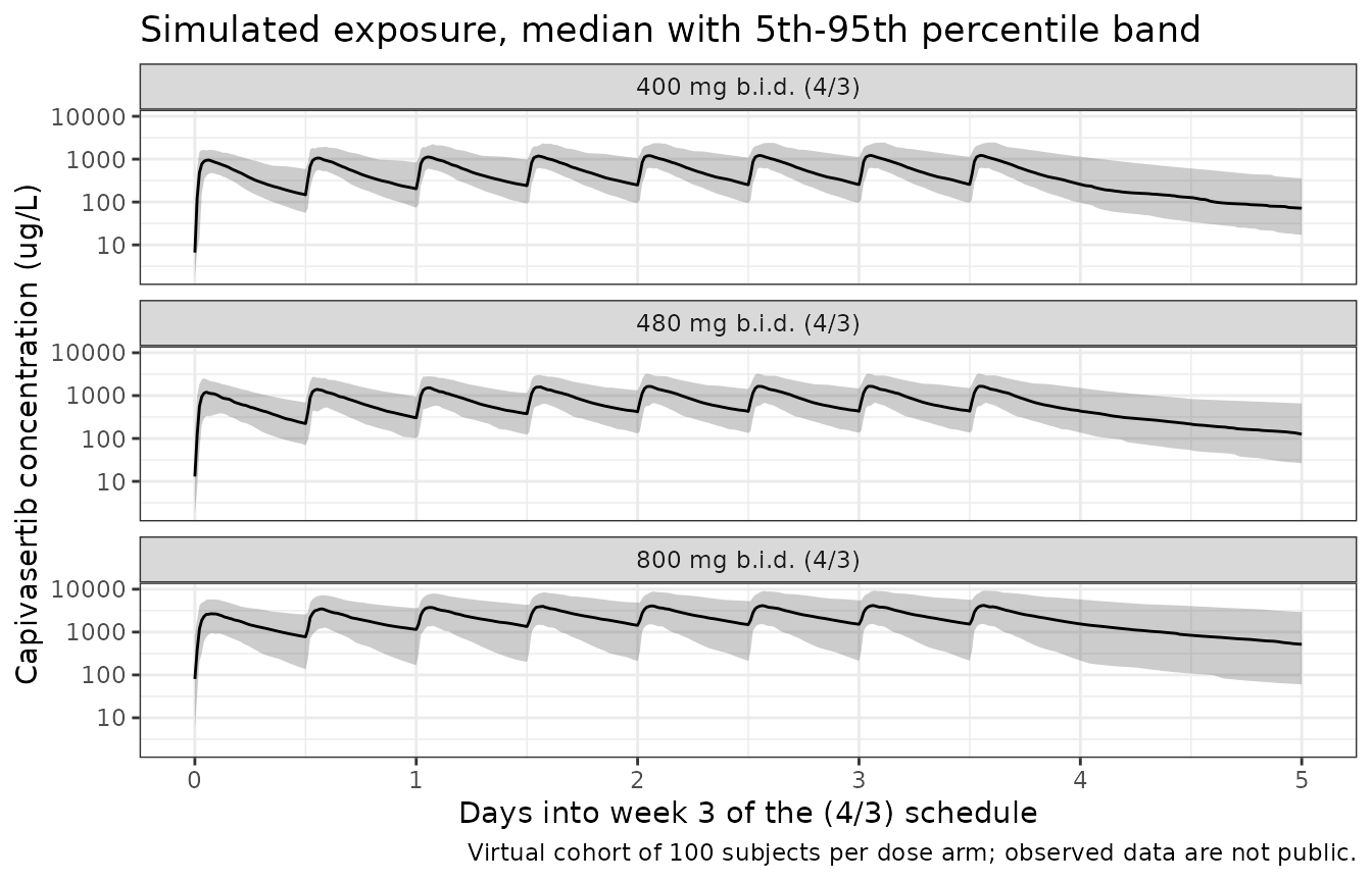
PKNCA validation
sim_nca <- sim |>
  dplyr::filter(!is.na(Cc)) |>
  dplyr::select(id, time, Cc, treatment)

# The steady-state interval starts at ss_start, and the observation grid
# contains that exact time point, so PKNCA has an anchor at the interval start.
stopifnot(any(abs(obs_grid - ss_start) < 1e-9),
          any(abs(obs_grid - ss_end)   < 1e-9))

dose_df <- events |>
  dplyr::filter(evid == 1, cmt == "depot") |>
  dplyr::select(id, time, amt, treatment)

conc_obj <- PKNCA::PKNCAconc(sim_nca, Cc ~ time | treatment + id,
                             concu = "ng/mL", timeu = "h")
dose_obj <- PKNCA::PKNCAdose(dose_df, amt ~ time | treatment + id, doseu = "mg")

intervals <- data.frame(
  start   = ss_start,
  end     = ss_end,
  cmax    = TRUE,
  tmax    = TRUE,
  auclast = TRUE,
  cav     = TRUE
)

nca_res <- PKNCA::pk.nca(PKNCA::PKNCAdata(conc_obj, dose_obj, intervals = intervals))
nca_tbl <- as.data.frame(nca_res$result)
stopifnot(nrow(nca_tbl) > 0, !anyNA(nca_tbl$PPORRES))

nca_tbl |>
  group_by(treatment, PPTESTCD) |>
  summarise(Median = median(PPORRES), `5th pctile` = quantile(PPORRES, 0.05),
            `95th pctile` = quantile(PPORRES, 0.95), .groups = "drop") |>
  mutate(Parameter = nlmixr2lib::ncaParamLabel(PPTESTCD), .before = PPTESTCD) |>
  select(-PPTESTCD) |>
  knitr::kable(digits = 1, caption = paste(
    "Steady-state NCA over the week-3, 4th-dosing-day interval",
"(", ss_start, "-", ss_end, "h), full between-subject variability."))| treatment | Parameter | Median | 5th pctile | 95th pctile |
|---|---|---|---|---|
| 400 mg b.i.d. (4/3) | AUClast | 7943.9 | 4308.3 | 17818.8 |
| 400 mg b.i.d. (4/3) | Cavg | 662.0 | 359.0 | 1484.9 |
| 400 mg b.i.d. (4/3) | Cmax | 1375.6 | 724.3 | 2492.4 |
| 400 mg b.i.d. (4/3) | Tmax | 1.2 | 0.5 | 2.8 |
| 480 mg b.i.d. (4/3) | AUClast | 10456.6 | 5126.7 | 21039.2 |
| 480 mg b.i.d. (4/3) | Cavg | 871.4 | 427.2 | 1753.3 |
| 480 mg b.i.d. (4/3) | Cmax | 1646.0 | 831.5 | 3134.5 |
| 480 mg b.i.d. (4/3) | Tmax | 1.5 | 0.8 | 3.2 |
| 800 mg b.i.d. (4/3) | AUClast | 26034.8 | 14024.7 | 71578.7 |
| 800 mg b.i.d. (4/3) | Cavg | 2169.6 | 1168.7 | 5964.9 |
| 800 mg b.i.d. (4/3) | Cmax | 3876.3 | 2140.5 | 8511.1 |
| 800 mg b.i.d. (4/3) | Tmax | 1.5 | 0.8 | 3.5 |
Comparison against published NCA
Fernandez-Teruel 2024 Sect. 3.5 reports median AUC12h,ss
of 7730 ug*h/L and median Cmax,ss of 1340 ug/L at 400 mg
b.i.d. (4/3), and Sect. 3.2 gives a steady-state Tmax of
about 1.4 h. Those values are compared here against the
typical-value profile – see the note in Assumptions and deviations for
why the full-variability cohort median sits above them.
tv_events <- make_events(1L, 400, dose_times("4/3", 3L),
                         seq(ss_start, ss_end, by = 0.02),
                         treatment = "400 mg b.i.d. (4/3)")
tv_sim <- as.data.frame(rxode2::rxSolve(tv, tv_events, keep = "treatment",
                                        addDosing = FALSE))
#> ℹ omega/sigma items treated as zero: 'etalcl', 'etalvc', 'etalcl_time_max', 'etaltlag', 'etalogitffo', 'etalka', 'etald1'
# rxSolve omits the `id` column entirely for a single-subject event table;
# PKNCA's grouping formula needs it back.
if (is.null(tv_sim$id)) tv_sim$id <- 1L

tv_conc <- PKNCA::PKNCAconc(
  tv_sim |> filter(!is.na(Cc)) |> select(id, time, Cc, treatment),
  Cc ~ time | treatment + id, concu = "ng/mL", timeu = "h")
tv_dose <- PKNCA::PKNCAdose(
  tv_events |> filter(evid == 1, cmt == "depot") |> select(id, time, amt, treatment),
  amt ~ time | treatment + id, doseu = "mg")
tv_res <- PKNCA::pk.nca(PKNCA::PKNCAdata(
  tv_conc, tv_dose,
  intervals = data.frame(start = ss_start, end = ss_end,
                         cmax = TRUE, tmax = TRUE, auclast = TRUE)))

published <- tibble::tibble(
  treatment = "400 mg b.i.d. (4/3)",
  cmax = 1340, tmax = 1.4, auclast = 7730
)

cmp <- nlmixr2lib::ncaComparisonTable(
  simulated = tv_res, reference = published, by = "treatment",
  units = c(cmax = "ug/L", tmax = "h", auclast = "ug*h/L"),
  tolerance_pct = 20
)
knitr::kable(cmp, caption = paste(
  "Typical-value steady-state NCA versus the values Fernandez-Teruel 2024",
  "reports. * marks a difference above 20%."),
align = c("l", "l", "r", "r", "r"))| NCA parameter | treatment | Reference | Simulated | % diff |
|---|---|---|---|---|
| Cmax (ug/L) | 400 mg b.i.d. (4/3) | 1340 | 1350 | +1.0% |
| Tmax (h) | 400 mg b.i.d. (4/3) | 1.4 | 1.4 | -0.0% |
| AUClast (ug*h/L) | 400 mg b.i.d. (4/3) | 7730 | 7690 | -0.5% |
Verification summary
summary_tbl <- dplyr::bind_rows(acc$rows) |>
  mutate(`Abs. difference` = abs(Reproduced - Published)) |>
  select(Quantity, Unit, Published, Reproduced, `Abs. difference`,
         Tolerance, Pass, Deviation)

summary_tbl |>
  mutate(across(c(Published, Reproduced, `Abs. difference`, Tolerance),
                ~ signif(.x, 4))) |>
  knitr::kable(caption = paste(
    "Every published quantity checked against the packaged model. Rows marked",
"Deviation = TRUE are discussed in Assumptions and deviations."))| Quantity | Unit | Published | Reproduced | Abs. difference | Tolerance | Pass | Deviation |
|---|---|---|---|---|---|---|---|
| Apparent volume of distribution at steady state (Vss = V2 + V3 + V4) | L | 255.60 | 255.6000 | 0.000e+00 | 0.20 | TRUE | FALSE |
| Fraction of the dose absorbed by the first-order route at 67 kg | fraction | 0.80 | 0.8022 | 2.184e-03 | 0.01 | TRUE | FALSE |
| Disposition half-life t1/2-alpha, first dose | h | 0.37 | 0.3699 | 5.340e-05 | 0.05 | TRUE | FALSE |
| Disposition half-life t1/2-alpha, multiple doses at 400 mg | h | 0.42 | 0.4145 | 5.489e-03 | 0.05 | TRUE | FALSE |
| Disposition half-life t1/2-beta, first dose | h | 4.20 | 4.1560 | 4.356e-02 | 0.20 | TRUE | FALSE |
| Disposition half-life t1/2-beta, multiple doses at 400 mg | h | 4.40 | 4.3880 | 1.223e-02 | 0.20 | TRUE | FALSE |
| Disposition half-life t1/2-gamma, first dose | h | 31.00 | 30.7800 | 2.212e-01 | 1.00 | TRUE | FALSE |
| Disposition half-life t1/2-gamma, multiple doses at 400 mg | h | 31.00 | 31.0500 | 5.371e-02 | 1.00 | TRUE | FALSE |
| Tmax at steady state, 400 mg b.i.d. (4/3) | h | 1.40 | 1.4000 | 0.000e+00 | 0.15 | TRUE | FALSE |
| AUC12,ss, 400 mg b.i.d. (4/3) | ug*h/L | 7730.00 | 7693.0000 | 3.690e+01 | 300.00 | TRUE | FALSE |
| Cmax,ss, 400 mg b.i.d. (4/3) | ug/L | 1340.00 | 1353.0000 | 1.344e+01 | 70.00 | TRUE | FALSE |
| Accumulation ratio, 400 mg b.i.d. (4/3) | ratio | 1.58 | 1.5800 | 1.097e-04 | 0.05 | TRUE | FALSE |
| Effective half-life, 400 mg b.i.d. (4/3) | h | 8.34 | 8.2990 | 4.109e-02 | 0.40 | TRUE | FALSE |
| Reduction in CL/F at 120 h, 400 mg | % | 18.00 | 16.2100 | 1.795e+00 | 4.50 | TRUE | TRUE |
| Reduction in CL/F at 120 h, 480 mg | % | 22.00 | 20.3000 | 1.697e+00 | 4.50 | TRUE | TRUE |
| Reduction in CL/F at 120 h, 800 mg | % | 54.00 | 50.0300 | 3.971e+00 | 4.50 | TRUE | TRUE |
| AUC12,ss ratio - Body weight 47 kg | ratio | 1.14 | 1.1320 | 8.000e-03 | 0.03 | TRUE | FALSE |
| Cmax,ss ratio - Body weight 47 kg | ratio | 1.14 | 1.1420 | 2.000e-03 | 0.03 | TRUE | FALSE |
| AUC12,ss ratio - Concomitant paclitaxel | ratio | 0.84 | 0.8490 | 9.000e-03 | 0.03 | TRUE | FALSE |
| Cmax,ss ratio - Concomitant paclitaxel | ratio | 0.89 | 0.8980 | 8.000e-03 | 0.03 | TRUE | FALSE |
Assumptions and deviations
Imaxis on the log scale. Fernandez-Teruel 2024 never says so in words, and its Table 3 row is labelled “Imax” with no unit. The reading is forced by equation (e), which placesImax_iinside an exponential, and it is confirmed four times over: it reproduces the reported 18% / 22% / 54% reductions inCL/F, the +20%CLss/Fwith paclitaxel, the 7730 ug*h/LAUC12,ss, and the 1340 ug/LCmax,ss. The alternative reading –-1.54as a fraction – would make clearance rise by 154% over time and is excluded by every one of those.The auto-inhibition reproduces about 1-2 percentage points shallower than published, and this is left as-is. Using Table 3’s printed
Imax = -1.54the model gives maximal reductions of 17.1% / 21.4% / 52.8% at 400 / 480 / 800 mg against the published 18% / 22% / 54%; at exactly 120 h the figures are 16.2% / 20.3% / 50.0%. AnImaxof about -1.50 would reproduce all three to within 0.3 points, and -1.50 sits comfortably inside the paper’s own bootstrap interval of -1.85 to -1.29 (bootstrap median -1.51). The published percentages were read off the Fig. 4 simulation rather than tabulated, so the residual is consistent with rounding the point estimate to three significant figures. No parameter was tuned: the file keeps -1.54 exactly as printed and the summary table flags these three rows as a known deviation.Between-subject variability is read as
omega = CV / 100. Table 3 reports every BSV as a percent coefficient of variation, includingLogit F1, whose random effect Sect. 3.2 describes as additive. A CV is only interpretable as100 * sqrt(omega^2)for an additive random effect, so that convention – and not the log-normalCV = 100 * sqrt(exp(omega^2) - 1)– is applied uniformly. Under the alternative convention the log-normal omegas would be smaller (for example V2/F would be 0.913 rather than 1.14) while the additive one would be unchanged, which would make the table internally inconsistent.The full-variability cohort median exceeds the published median by about 12-17% for AUC, while the typical-value profile matches it to within 0.5%. This follows from where the paper puts the random effect on
Imax: equation (f) multiplies a negative log-scale quantity byexp(eta), an asymmetric transform. A subject witheta = -0.706(one SD below) gets a 42% maximal reduction inCL/F, whereas one ateta = +0.706gets only 3%; the downside is far larger than the upside, so the cohort’s clearance distribution is skewed low and its exposure distribution skewed high. That is a faithful property of the published parameterisation, not an encoding choice, so the comparison against the paper’s reportedAUC12,ss/Cmax,ss/Tmaxis made on the typical-value profile and the cohort NCA is reported descriptively.Residual error is rendered on the linear scale. Sect. 3.2 states the model was fitted to log-transformed data with a combined proportional and additive residual error. nlmixr2’s
Cc ~ prop(propSd) + add(addSd)is the linear-scale equivalent, withpropSd = 0.439(the reported 43.9% CV) andaddSd = 0.504 ng/mL(the reported 0.504 ug/L; 1 ug/L = 1 ng/mL).Steady-state window. The paper predicts steady state “on every third and fourth dosing day each week from the second week” under the (4/3) schedule (Sect. 3.2). The 12 h interval used throughout this vignette is the fourth dosing day of week three (408-420 h). Choosing the third dosing day instead lowers
AUC12,ssby about 2%.Covariates screened but not retained. Fernandez-Teruel 2024 tested age, sex, race, creatinine clearance, hepatic function, renal function, smoking status, schedule, and concomitant fulvestrant, CYP3A inducers, CYP3A inhibitors and acid-reducing agents, and retained none of them. They carry no published point estimate and so cannot be encoded; they are recorded in the model file’s
covariatesDataExcludedmetadata for provenance.Absorption-route dosing requires two records per administration. The parallel first-order / zero-order input is a single NONMEM dose duplicated across two compartments (
F1intodepot,F2 = 1 - F1intocentral). Event tables must therefore carry twoevid = 1rows per administration with the sameamt, and thecentralrow must setrate = -2so rxode2 uses the modelled durationD2. Themake_events()helper above shows the pattern.Virtual cohort demographics. Body weight is drawn log-normally with median 67 kg and truncated to the published 32-129 kg range; the paper reports the median and range but not the distributional form. Weight is the only covariate varied – formulation, prandial state and concomitant paclitaxel are held at the reference levels of the paper’s own forest plots.
Supplement. The Electronic Supplementary Material was not required: every final parameter estimate is in main-text Table 3, and every structural and covariate equation is in main-text Sect. 3.3. The ESM holds the per-study dose and sampling schedules (Table 1), additional baseline covariates (Table 2), the VPCs (Figs. 1-2), the
CLss/Fforest plot (Fig. 3) and the in vitro kinase-inhibition results (Figs. 4-9, Tables 4-7). ```