Hydroxychloroquine and three metabolites (Alvarez 2022)
Source:vignettes/articles/Alvarez_2022_hydroxychloroquine.Rmd
Alvarez_2022_hydroxychloroquine.RmdModel and source
mod <- rxode2::rxode(readModelDb("Alvarez_2022_hydroxychloroquine"))
#> ℹ parameter labels from comments will be replaced by 'label()'
th <- mod$theta- Citation: Alvarez JC, Davido B, Moine P, Etting I, Annane D, Larabi IA, Simon N (2022). Population Pharmacokinetics of Hydroxychloroquine and 3 Metabolites in COVID-19 Patients and Pharmacokinetic/Pharmacodynamic Application. Pharmaceuticals 15(2):256. doi:10.3390/ph15020256.
- Article: https://doi.org/10.3390/ph15020256
- PMCID: PMC8877570
Joint parent + three-metabolite population PK model for oral hydroxychloroquine in whole blood of 100 adults hospitalised with COVID-19 (medicine wards and ICU) (Alvarez 2022). One-compartment hydroxychloroquine disposition with first-order absorption and a lag time (both fixed to published values), a non-metabolic apparent clearance, and three parallel first-order formation clearances into one-compartment desethylhydroxychloroquine, desethylchloroquine and bisdesethylchloroquine (didesethylchloroquine) compartments whose volumes equal the individual hydroxychloroquine volume. Formation fluxes carry a molar correction so each metabolite state holds mg of that metabolite. No covariates were retained (age, weight, height, BMI, sex, azithromycin co-treatment and ICU stay were screened). Proportional plus additive residual error on every analyte.
Population
| Field | Value |
|---|---|
| species | human |
| n_subjects | 100 |
| n_studies | 1 |
| n_observations | 333 whole-blood samples, each assayed for hydroxychloroquine and the three metabolites; 1 to 9 samples per patient (Section 2.1.1) |
| age_range | 20-94 years (mean 60.7, SD 15.9; median 62.5) |
| weight_range | 37.5-190 kg (mean 83.6, SD 20.1; median 82) |
| sex_female_pct | 34 |
| disease_state | Hospitalised COVID-19 confirmed by SARS-CoV-2 RT-PCR and/or compatible chest CT; 75 on medicine wards, 25 in the ICU |
| dose_range | Plaquenil 200 mg bid or tid orally, preceded in 42 patients by a 400 mg bid loading dose on day 1 |
| regions | France (Raymond Poincare Hospital, Garches) |
| co_medication | Azithromycin in 78 patients |
| notes | Retrospective therapeutic drug monitoring cohort; samples roughly every two days over the first two weeks of treatment (Figure 2). |
One hundred adults hospitalised with COVID-19 at Raymond Poincare Hospital (Garches, France), 75 on medicine wards and 25 in the intensive care unit, were treated with oral hydroxychloroquine (Plaquenil 200 mg) at 200 mg twice or three times daily, in 42 patients after a 400 mg twice-daily loading day, and 78 also received azithromycin (Table 1, Section 4.1). Whole-blood hydroxychloroquine (HCQ), desethylhydroxychloroquine (DHCQ; the paper’s DesHCQ or DesOHCQ), desethylchloroquine (DCQ; DesCQ) and bisdesethylchloroquine (BDCQ; DiDesCQ) were measured by LC-MS/MS in 333 samples, 1 to 9 per patient, collected roughly every two days as therapeutic drug monitoring.
Model structure
Figure 3 of the paper: hydroxychloroquine is absorbed first-order after a lag into a single central compartment (VP/F) and leaves it by four parallel clearances – its own apparent clearance CL/F and three formation clearances, one into each metabolite compartment. Each metabolite has its own first-order elimination clearance and a volume fixed to the individual parent volume. The model was fitted in NONMEM (ADVAN5, FOCE-I) on molar concentrations, so each metabolite is formed 1:1 in moles; the packaged model keeps doses in mg and multiplies each formation flux by the metabolite-to-parent molecular-weight ratio, so every compartment holds mg of its own analyte and every output is in ug/L.
The paper reports that 75% of hydroxychloroquine is converted to the metabolites, computed as the sum of formation clearances over the total (Section 2.1.1). The packaged values reproduce it:
Source trace
| Item | Value | Source |
|---|---|---|
| Structure: 1-cmt HCQ, 3 parallel 1-cmt metabolites | - | Figure 3; Section 2.1.1 |
| Metabolite volume = parent volume VP/F | - | Section 2.1.1 |
| Molar concentrations in the fit | - | Section 4.3 |
| tlag (fixed) | 0.389 h | Table 2 (from Lim 2009, reference 16) |
| ka (fixed) | 1.15 1/h | Table 2 (from Lim 2009, reference 16) |
| cl (CL/F HCQ) | 5.60 L/h | Table 2 |
| vc (VP/F HCQ) | 1850 L | Table 2 |
| cl_form_dhcq (CL HCQ_DesHCQ) | 9.63 L/h | Table 2 |
| cl_form_dcq (CL HCQ_DesCQ) | 4.99 L/h | Table 2 |
| cl_form_bdcq (CL HCQ_DiDesCQ) | 1.84 L/h | Table 2 |
| cl_dhcq (CL DesHCQ) | 8.89 L/h | Table 2 |
| cl_dcq (CL DesCQ) | 49.8 L/h | Table 2 |
| cl_bdcq (CL DiDesCQ) | 11.6 L/h | Table 2 |
| IIV CL, VP, CL DesHCQ, CL DesCQ, CL DiDesCQ | 1.327, 0.889, 0.860, 0.362, 0.953 | Table 2 (entered as variances; see below) |
| Proportional residual HCQ / DHCQ / DCQ / BDCQ | 0.448 / 0.428 / 0.322 / 0.0574 | Table 2 |
| Additive residual HCQ / DHCQ / DCQ / BDCQ | 86.9 / 6.69 / 5.78 / 2.49 ug/L | Table 2 |
| Fraction metabolised | 75% | Section 2.1.1 |
Deterministic checks
A single 200 mg dose is solved with the random effects zeroed over
3000 h, long enough for the slowest analyte (desethylhydroxychloroquine,
elimination half-life log(2) * 1850 / 8.89 = 144 h) to fall
more than twenty half-lives.
mod_typ <- rxode2::zeroRe(mod)
tgrid <- sort(unique(c(seq(0, 12, by = 0.25), seq(12, 96, by = 1), seq(96, 3000, by = 6))))
ev_single <- dplyr::bind_rows(
  data.frame(id = 1, time = 0, evid = 1, amt = 200, cmt = "depot", dvid = NA_integer_),
  data.frame(id = 1, time = tgrid, evid = 0, amt = 0, cmt = "central", dvid = 1L)
) |>
  dplyr::mutate(treatment = "200 mg single dose")
sim_single <- rxode2::rxSolve(mod_typ, events = ev_single, rtol = 1e-10, atol = 1e-12,
                              maxsteps = 1e6, keep = "treatment") |>
  as.data.frame() |>
  # A single-subject solve returns no id column.
  dplyr::mutate(id = 1L)
#> ℹ omega/sigma items treated as zero: 'etalcl', 'etalvc', 'etalcl_dhcq', 'etalcl_dcq', 'etalcl_bdcq'
Mass balance (PKNCA)
At infinite time the amount cleared equals the amount that entered.
For the parent, (CL/F + sum CL_form) * AUCinf = Dose; for
each metabolite,
CL_m * AUCinf_m = Dose * CL_form_m / CL_total * MW_m / MW_HCQ.
These close only if every clearance, the shared volume and each molar
correction are wired correctly.
analytes <- c(Cc = "HCQ", Cc_dhcq = "DHCQ", Cc_dcq = "DCQ", Cc_bdcq = "BDCQ")
peak <- vapply(names(analytes), function(v) max(sim_single[[v]]), numeric(1))
# The numeric (ODE) path can undershoot zero by about atol in the far tail.
for (v in names(analytes)) {
  stopifnot(all(sim_single[[v]] >= -1e-6 * peak[[v]]))
}

conc_long <- sim_single |>
  dplyr::select(id, time, treatment, dplyr::all_of(names(analytes))) |>
  tidyr::pivot_longer(dplyr::all_of(names(analytes)), names_to = "var", values_to = "Cc") |>
  dplyr::mutate(analyte = unname(analytes[var]), Cc = pmax(Cc, 0)) |>
  dplyr::filter(!is.na(Cc))
# Guarantee a time-zero record per analyte; any existing time-zero row wins.
conc_long <- dplyr::bind_rows(
  conc_long,
  conc_long |> dplyr::distinct(id, treatment, analyte) |> dplyr::mutate(time = 0, Cc = 0)
) |>
  dplyr::distinct(id, treatment, analyte, time, .keep_all = TRUE) |>
  dplyr::arrange(analyte, id, time)

dose_long <- ev_single |>
  dplyr::filter(evid == 1) |>
  dplyr::select(id, time, amt, treatment) |>
  tidyr::crossing(analyte = unname(analytes))

conc_obj <- PKNCA::PKNCAconc(as.data.frame(conc_long), Cc ~ time | treatment + analyte + id,
                             concu = "ug/L", timeu = "h")
dose_obj <- PKNCA::PKNCAdose(as.data.frame(dose_long), amt ~ time | treatment + analyte + id,
                             doseu = "mg")
intervals <- data.frame(start = 0, end = Inf, cmax = TRUE, tmax = TRUE,
                        aucinf.obs = TRUE, half.life = TRUE)
nca_res <- PKNCA::pk.nca(PKNCA::PKNCAdata(conc_obj, dose_obj, intervals = intervals))
nca_tab <- as.data.frame(nca_res$result)
mw <- c(HCQ = 335.87, DHCQ = 307.82, DCQ = 291.82, BDCQ = 263.77)
cl_out <- c(HCQ = cl_tot, DHCQ = exp(th[["lcl_dhcq"]]), DCQ = exp(th[["lcl_dcq"]]),
            BDCQ = exp(th[["lcl_bdcq"]]))
frac_in <- c(HCQ = 1, DHCQ = cl_form[["lcl_form_dhcq"]] / cl_tot,
             DCQ = cl_form[["lcl_form_dcq"]] / cl_tot, BDCQ = cl_form[["lcl_form_bdcq"]] / cl_tot)

mb <- nca_tab |>
  dplyr::filter(PPTESTCD == "aucinf.obs") |>
  dplyr::select(analyte, auc = PPORRES) |>
  dplyr::mutate(
    cleared_mg = cl_out[analyte] * auc / 1000,
    expected_mg = 200 * frac_in[analyte] * mw[analyte] / mw[["HCQ"]],
    ratio = cleared_mg / expected_mg
  )
stopifnot(nrow(mb) == 4L, setequal(mb$analyte, unname(analytes)))
mb |>
  dplyr::rename("Analyte" = analyte, "AUCinf (ug*h/L)" = auc, "CL x AUCinf (mg)" = cleared_mg,
                "Expected (mg)" = expected_mg, "Ratio" = ratio) |>
  knitr::kable(digits = c(0, 0, 3, 3, 4),
caption = "Mass balance after a single 200 mg dose (typical values).")| Analyte | AUCinf (ug*h/L) | CL x AUCinf (mg) | Expected (mg) | Ratio |
|---|---|---|---|---|
| BDCQ | 1129 | 13.100 | 13.101 | 0.9999 |
| DCQ | 789 | 39.304 | 39.307 | 0.9999 |
| DHCQ | 9000 | 80.012 | 80.016 | 0.9999 |
| HCQ | 9066 | 200.007 | 200.000 | 1.0000 |
Terminal half-lives
The parent’s terminal half-life is
log(2) * VP / CL_total. A metabolite whose elimination is
slower than the parent’s shows its own half-life
(log(2) * VP / CL_m); desethylchloroquine is eliminated
faster than it is formed, so its terminal phase follows the parent
(formation-rate-limited).
vc_typ <- exp(th[["lvc"]])
t12_parent <- log(2) * vc_typ / cl_tot
t12_expected <- c(
  HCQ = t12_parent,
  DHCQ = max(t12_parent, log(2) * vc_typ / cl_out[["DHCQ"]]),
  DCQ = max(t12_parent, log(2) * vc_typ / cl_out[["DCQ"]]),
  BDCQ = max(t12_parent, log(2) * vc_typ / cl_out[["BDCQ"]])
)
hl <- nca_tab |>
  dplyr::filter(PPTESTCD == "half.life") |>
  dplyr::select(analyte, half_life = PPORRES) |>
  dplyr::mutate(expected = t12_expected[analyte], pct_diff = 100 * (half_life / expected - 1))
stopifnot(nrow(hl) == 4L)
hl |>
  dplyr::rename("Analyte" = analyte, "PKNCA t1/2 (h)" = half_life,
                "Closed-form t1/2 (h)" = expected, "Difference (%)" = pct_diff) |>
knitr::kable(digits = c(0, 1, 1, 2), caption = "Terminal half-life after a single dose.")| Analyte | PKNCA t1/2 (h) | Closed-form t1/2 (h) | Difference (%) |
|---|---|---|---|
| BDCQ | 111.3 | 110.5 | 0.65 |
| DCQ | 58.4 | 58.1 | 0.51 |
| DHCQ | 145.1 | 144.2 | 0.57 |
| HCQ | 58.1 | 58.1 | 0.00 |
# Deterministic. PKNCA picks its own lambda-z window, which for the
# formation-limited DCQ and the slow metabolites may still carry a trace of the
# faster exponential; 3% separates that from a wrong clearance or volume.
stopifnot(all(abs(hl$pct_diff) < 3))
The paper’s parent volume of 1850 L gives a parent half-life of about 58 h (2.4 days) within this model. The Discussion’s “more than 40 days” terminal half-life is quoted from the literature on long-term treatment and is not a property of the fitted one-compartment model, which was estimated on the first two weeks of therapy.
Replication of Figure 8 (trough concentrations at 48 h and 72 h)
Figure 8 simulated 500 patients per regimen “with between subject variability” and shows boxplots of the hydroxychloroquine whole-blood trough at 48 h and 72 h after the first dose for five regimens. The maintainers digitised the quartiles of each box from the published raster (the pixel scale was read from the 0, 600, 800, 1000 and 2000 ug/L gridlines). The trough is taken just before the dose due at that time.
To compare quartiles without Monte Carlo noise, the model’s trough distribution is computed on a fixed lattice rather than a random cohort. Only two random effects move the parent trough (CL/F and VP/F; the metabolite etas do not act on the parent), so 14 equally probable quantiles of each give 196 lattice patients per regimen, and each of their predictions is crossed with a 20 x 20 lattice of the proportional and additive residual draws. Every number in the tables of this section is therefore deterministic.
fig8 <- tibble::tribble(
  ~scenario, ~time, ~q25, ~q50, ~q75,
  "1: 200 mg bid", 48, 115, 251, 399,
  "1: 200 mg bid", 72, 158, 339, 546,
  "2: 200 mg tid", 48, 210, 369, 615,
  "2: 200 mg tid", 72, 235, 456, 757,
  "3: 400 mg bid day 1, then 200 mg bid", 48, 194, 339, 593,
  "3: 400 mg bid day 1, then 200 mg bid", 72, 199, 396, 617,
  "4: 400 mg bid day 1, then 200 mg tid", 48, 210, 410, 719,
  "4: 400 mg bid day 1, then 200 mg tid", 72, 243, 473, 757,
  "5: 400 mg bid", 48, 240, 484, 803,
  "5: 400 mg bid", 72, 284, 557, 1022
)

bid <- seq(0, 60, by = 12)
tid <- seq(0, 64, by = 8)
regimens <- list(
  "1: 200 mg bid" = data.frame(time = bid, amt = 200),
  "2: 200 mg tid" = data.frame(time = tid, amt = 200),
  "3: 400 mg bid day 1, then 200 mg bid" = data.frame(time = bid, amt = ifelse(bid < 24, 400, 200)),
  "4: 400 mg bid day 1, then 200 mg tid" = data.frame(time = c(0, 12, seq(24, 64, by = 8)),
                                                      amt = c(400, 400, rep(200, 6))),
  "5: 400 mg bid" = data.frame(time = bid, amt = 400)
)
trough_events <- function(n_per_arm) {
  dplyr::bind_rows(lapply(seq_along(regimens), function(i) {
    ids <- (i - 1) * n_per_arm + seq_len(n_per_arm)
    dplyr::bind_rows(
      tidyr::crossing(id = ids, regimens[[i]]) |>
        dplyr::mutate(evid = 1, cmt = "depot", dvid = NA_integer_),
      tidyr::crossing(id = ids, time = c(48, 72)) |>
        dplyr::mutate(evid = 0, amt = 0, cmt = "central", dvid = 1L)
    ) |>
      dplyr::mutate(scenario = names(regimens)[i], lattice = seq_len(n_per_arm)[match(id, ids)])
  })) |>
    dplyr::arrange(id, time, dplyr::desc(evid))
}

# Equally probable standard-normal quantiles, rescaled to unit variance so the
# lattice does not understate the spread.
lattice_z <- function(n) {
  z <- stats::qnorm((seq_len(n) - 0.5) / n)
  z / sqrt(mean(z^2))
}
eta_grid <- expand.grid(z_cl = lattice_z(14), z_v = lattice_z(14))
eps_grid <- expand.grid(e_prop = lattice_z(20), e_add = lattice_z(20))
ev_lat <- trough_events(nrow(eta_grid))
stopifnot(dplyr::n_distinct(ev_lat$id) == 5 * nrow(eta_grid))
# Typical-value model; the lattice supplies the individual CL/F and VP/F.
solve_lattice <- function(omega_cl, omega_v) {
  ids <- dplyr::distinct(ev_lat, id, lattice)
  prm <- data.frame(
    id = ids$id,
    lcl = th[["lcl"]] + sqrt(omega_cl) * eta_grid$z_cl[ids$lattice],
    lvc = th[["lvc"]] + sqrt(omega_v) * eta_grid$z_v[ids$lattice]
  )
  rxode2::rxSolve(mod_typ, params = prm, events = ev_lat, keep = "scenario") |>
    as.data.frame() |>
    dplyr::select(id, scenario, time, Cc)
}
with_ruv <- function(pred, prop_sd, add_sd = th[["addSd"]]) {
  tidyr::crossing(pred, eps_grid) |>
    dplyr::mutate(Cobs = Cc * (1 + prop_sd * e_prop) + add_sd * e_add)
}
quartiles <- function(d, conc) {
  d |>
    dplyr::group_by(scenario, time) |>
    dplyr::summarise(
      sim_q25 = stats::quantile(.data[[conc]], 0.25),
      sim_q50 = stats::quantile(.data[[conc]], 0.50),
      sim_q75 = stats::quantile(.data[[conc]], 0.75),
      pct_below_200 = 100 * mean(.data[[conc]] < 200),
      .groups = "drop"
    ) |>
    dplyr::inner_join(fig8, by = c("scenario", "time"))
}

# Packaged reading: the Table 2 values are the omega variances.
om_cl <- mod$omega["etalcl", "etalcl"]
om_v <- mod$omega["etalvc", "etalvc"]
stopifnot(om_cl == 1.327, om_v == 0.889)
pred_var <- solve_lattice(om_cl, om_v)
#> ℹ omega/sigma items treated as zero: 'etalcl', 'etalvc', 'etalcl_dhcq', 'etalcl_dcq', 'etalcl_bdcq'
#> Warning: multi-subject simulation without without 'omega'
stopifnot(nrow(pred_var) == 2 * 5 * nrow(eta_grid), all(is.finite(pred_var$Cc)))
cmp <- quartiles(with_ruv(pred_var, th[["propSd"]]), "Cobs") |>
  dplyr::mutate(log_ratio_median = log(sim_q50 / q50))
stopifnot(nrow(cmp) == 10L)

cmp |>
  dplyr::select(scenario, time, sim_q25, q25, sim_q50, q50, sim_q75, q75, pct_below_200) |>
  dplyr::rename("Scenario" = scenario, "Time (h)" = time,
                "Model Q1" = sim_q25, "Fig 8 Q1" = q25, "Model median" = sim_q50,
                "Fig 8 median" = q50, "Model Q3" = sim_q75, "Fig 8 Q3" = q75,
                "Model % < 200 ug/L" = pct_below_200) |>
knitr::kable(digits = 0, caption = "Model HCQ trough quartiles (ug/L, lattice) against the digitised Figure 8 quartiles.")| Scenario | Time (h) | Model Q1 | Fig 8 Q1 | Model median | Fig 8 median | Model Q3 | Fig 8 Q3 | Model % < 200 ug/L |
|---|---|---|---|---|---|---|---|---|
| 1: 200 mg bid | 48 | 126 | 115 | 253 | 251 | 422 | 399 | 40 |
| 1: 200 mg bid | 72 | 169 | 158 | 319 | 339 | 516 | 546 | 30 |
| 2: 200 mg tid | 48 | 203 | 210 | 388 | 369 | 656 | 615 | 25 |
| 2: 200 mg tid | 72 | 269 | 235 | 493 | 456 | 804 | 757 | 17 |
| 3: 400 mg bid day 1, then 200 mg bid | 48 | 182 | 194 | 344 | 339 | 566 | 593 | 28 |
| 3: 400 mg bid day 1, then 200 mg bid | 72 | 209 | 199 | 382 | 396 | 609 | 617 | 24 |
| 4: 400 mg bid day 1, then 200 mg tid | 48 | 228 | 210 | 431 | 410 | 720 | 719 | 21 |
| 4: 400 mg bid day 1, then 200 mg tid | 72 | 288 | 243 | 523 | 473 | 847 | 757 | 16 |
| 5: 400 mg bid | 48 | 261 | 240 | 492 | 484 | 824 | 803 | 18 |
| 5: 400 mg bid | 72 | 344 | 284 | 626 | 557 | 1015 | 1022 | 12 |
# Deterministic (lattice, no random draw). Entering the dose as mg of the
# sulfate salt converted to base (x 0.774) moves every median by -0.26 on the
# log scale, a mis-scaled volume or a lost dose by more, so a 0.1 bound on the
# centre separates the packaged model from each of those.
stopifnot(
  abs(median(cmp$log_ratio_median)) < 0.1,
  median(abs(cmp$log_ratio_median)) < 0.1
)
The median absolute log-ratio between the model and the published medians is 0.05 across the ten boxes. The paper states that every regimen except 200 mg twice daily leaves fewer than 25% of patients below 200 ug/L. The model percentages are in the last column: scenarios 2 and 3 at 48 h sit at or just above 25%, and the published boxes themselves put scenario 3 at 48 h on that line (lower quartile 194 ug/L).
A random 200-patient cohort per regimen, with residual error, shown against the digitised quartiles:
rxode2::rxSetSeed(2022)
set.seed(2022)
sim_fig8 <- rxode2::rxSolve(mod, events = trough_events(200), keep = "scenario") |>
  as.data.frame()
sim_fig8$Cobs <- sim_fig8$Cc * (1 + th[["propSd"]] * stats::rnorm(nrow(sim_fig8))) +
  th[["addSd"]] * stats::rnorm(nrow(sim_fig8))

sim_fig8 |>
  dplyr::mutate(label = paste0("t", time, "h"), scenario = sub(":.*", "", scenario)) |>
  ggplot(aes(label, pmax(Cobs, 0))) +
  geom_boxplot(outlier.size = 0.5) +
  geom_point(data = fig8 |>
               tidyr::pivot_longer(c(q25, q50, q75), values_to = "conc") |>
               dplyr::mutate(label = paste0("t", time, "h"), scenario = sub(":.*", "", scenario)),
             aes(y = conc), colour = "red", shape = 4, size = 2.5) +
  facet_wrap(~scenario, nrow = 1, labeller = label_both) +
  coord_cartesian(ylim = c(0, 2500)) +
  labs(x = "Time since first administration", y = "HCQ blood trough (ug/L)",
       caption = "Boxes: 200 simulated patients per regimen. Red crosses: quartiles digitised from Figure 8.") +
  theme_bw()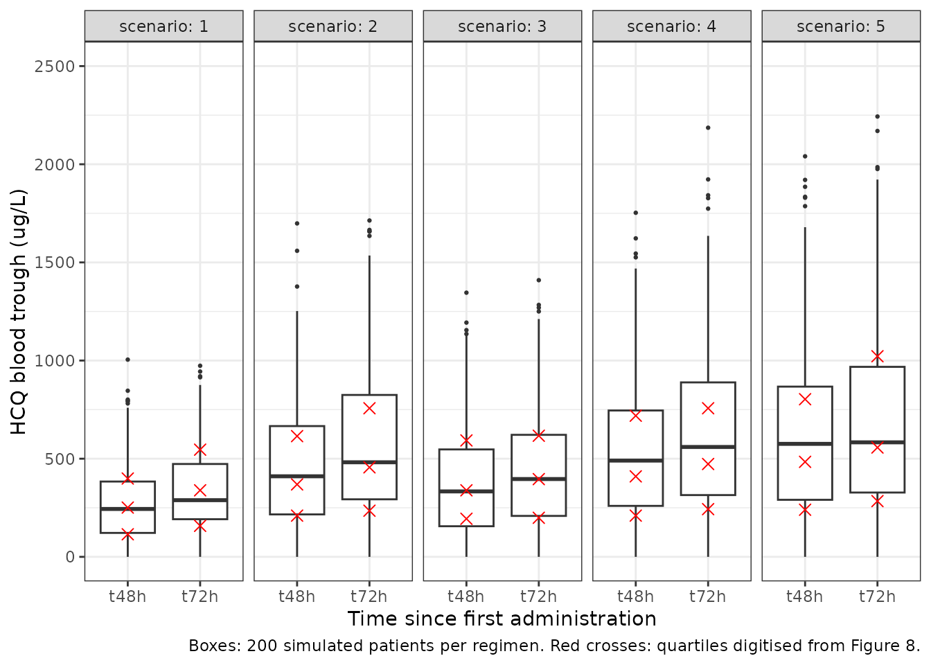
Replicates Figure 8 of Alvarez 2022.
What Figure 8 says about the dose unit and the variability scales
The paper leaves three things unstated: the molecular weight used to turn the dose into moles, and whether the Table 2 “omega” and “sigma” values are standard deviations or variances. Each reading is scored against Figure 8 on the same lattice:
score <- function(d, conc) {
  quartiles(d, conc) |>
    dplyr::summarise(
      q25 = mean(abs(log(pmax(sim_q25, 1) / q25))),
      q50 = mean(abs(log(sim_q50 / q50))),
      q75 = mean(abs(log(sim_q75 / q75)))
    )
}
# Alternative: the Table 2 values are SDs, so the variances are their squares.
pred_sd <- solve_lattice(om_cl^2, om_v^2)
#> ℹ omega/sigma items treated as zero: 'etalcl', 'etalvc', 'etalcl_dhcq', 'etalcl_dcq', 'etalcl_bdcq'
#> Warning: multi-subject simulation without without 'omega'
# The model is linear in dose, so a dose entered as sulfate salt (200 mg of
# salt = 200 * 335.87 / 433.95 mg of base) scales every prediction.
pred_salt <- dplyr::mutate(pred_var, Cc = Cc * 335.87 / 433.95)

scales <- dplyr::bind_rows(
  packaged = score(with_ruv(pred_var, th[["propSd"]]), "Cobs"),
  omega_sd = score(with_ruv(pred_sd, th[["propSd"]]), "Cobs"),
  sigma_var = score(with_ruv(pred_var, sqrt(th[["propSd"]])), "Cobs"),
  no_ruv = score(pred_var, "Cc"),
  salt = score(with_ruv(pred_salt, th[["propSd"]]), "Cobs"),
  .id = "reading"
)
reading_labels <- c(
  packaged = "Packaged: labelled mg, omega variances, sigma SDs",
  omega_sd = "Omega read as SDs",
  sigma_var = "Proportional sigma read as a variance",
  no_ruv = "No residual error",
  salt = "Dose read as mg of sulfate salt"
)
scales |>
  dplyr::mutate(reading = reading_labels[reading]) |>
  dplyr::rename("Reading" = reading, "Mean |log ratio| Q1" = q25,
                "Mean |log ratio| median" = q50, "Mean |log ratio| Q3" = q75) |>
knitr::kable(digits = 3, caption = "Distance of the model trough quartiles from Figure 8 under each reading (lattice).")| Reading | Mean |log ratio| Q1 | Mean |log ratio| median | Mean |log ratio| Q3 |
|---|---|---|---|
| Packaged: labelled mg, omega variances, sigma SDs | 0.097 | 0.053 | 0.045 |
| Omega read as SDs | 0.083 | 0.045 | 0.042 |
| Proportional sigma read as a variance | 0.181 | 0.046 | 0.072 |
| No residual error | 0.332 | 0.129 | 0.048 |
| Dose read as mg of sulfate salt | 0.193 | 0.213 | 0.227 |
sc <- function(r, q) {
  v <- scales[[q]][scales$reading == r]
  if (length(v) != 1L) stop("no unique score for ", r)
  v
}
# Deterministic. Each assertion is the claim written in the bullets below.
stopifnot(
  # The dose-unit reading separates by far more than any scale reading.
  sc("salt", "q50") > sc("packaged", "q50") + 0.1,
  # Figure 8 includes residual error: without it the lower quartiles miss badly.
  sc("no_ruv", "q25") > 2 * sc("packaged", "q25"),
  # The two omega readings are indistinguishable at 48-72 h.
  abs(sc("omega_sd", "q50") - sc("packaged", "q50")) < 0.02,
  abs(sc("omega_sd", "q25") - sc("packaged", "q25")) < 0.02,
  # A proportional SD of 0.448 fits the box widths better than 0.669.
  sc("sigma_var", "q25") + sc("sigma_var", "q75") > sc("packaged", "q25") + sc("packaged", "q75")
)- Dose unit. Plaquenil 200 mg tablets contain 200 mg of hydroxychloroquine sulfate. Converting the labelled 200 mg to moles with the free-base molecular weight reproduces the Figure 8 medians; treating it as sulfate salt (x 0.774 in moles) lowers every median by 23% and moves them away from the figure. The model therefore takes the labelled tablet strength in mg as the dose.
-
Omega. At 48 h and 72 h the trough is governed by
the volume (0.889 read as a variance is an SD of 0.943; read as an SD it
is 0.889) and hardly at all by the eta on the non-metabolic clearance.
The two readings’ scores differ by less than 0.02 on every quartile (the
SD reading is marginally closer), which is smaller than the uncertainty
from digitising the figure and from the unstated clock times of the
doses, so Figure 8 does not separate them. The values are entered as
variances because the same group’s companion lopinavir analysis (Alvarez
2021, identical table layout and “omega” labelling) was shown from its
own below-target percentages to report variances. The RSE column does
not decide it either: 9.2% on the CL row is below the floor a variance
estimated from 100 patients can reach (
sqrt(2/100)= 14%), but the lopinavir table’s variance rows sat below that floor too. The only row where the choice matters much is desethylchloroquine clearance (SD 0.60 versus 0.36). - Sigma. The additive terms carry concentration units (ug/L), so they are standard deviations. The proportional HCQ term read as an SD (0.448) fits the Figure 8 box widths better than read as a variance (SD 0.669), and without any residual error the lower quartiles are far too high, which shows that the figure includes residual error.
Four-analyte profiles over the first two weeks
Figure 2 of the paper shows the observed concentrations over the first 14 days. Two of the prescribed regimens are simulated for 200 patients each.
t_obs <- seq(0, 336, by = 4)
make_arm <- function(ids, doses, label) {
  dplyr::bind_rows(
    tidyr::crossing(id = ids, doses) |> dplyr::mutate(evid = 1, cmt = "depot", dvid = NA_integer_),
    tidyr::crossing(id = ids, time = t_obs) |>
      dplyr::mutate(evid = 0, amt = 0, cmt = "central", dvid = 1L)
  ) |>
    dplyr::mutate(treatment = label)
}
bid14 <- seq(0, 324, by = 12)
ev_prof <- dplyr::bind_rows(
  make_arm(1:200, data.frame(time = bid14, amt = 200), "200 mg bid"),
  make_arm(201:400, data.frame(time = bid14, amt = ifelse(bid14 < 24, 400, 200)),
           "400 mg bid day 1, then 200 mg bid")
) |>
  dplyr::arrange(id, time, dplyr::desc(evid))
rxode2::rxSetSeed(2025)
sim_prof <- rxode2::rxSolve(mod, events = ev_prof, keep = "treatment") |> as.data.frame()

prof_long <- sim_prof |>
  dplyr::select(id, time, treatment, dplyr::all_of(names(analytes))) |>
  tidyr::pivot_longer(dplyr::all_of(names(analytes)), names_to = "var", values_to = "conc") |>
  dplyr::mutate(analyte = factor(analytes[var], levels = unname(analytes)))
prof_summ <- prof_long |>
  dplyr::group_by(treatment, analyte, time) |>
  dplyr::summarise(
    p05 = stats::quantile(conc, 0.05), p50 = stats::median(conc), p95 = stats::quantile(conc, 0.95),
    .groups = "drop"
  )
ggplot(prof_summ, aes(time / 24, p50, colour = treatment, fill = treatment)) +
  geom_ribbon(aes(ymin = p05, ymax = p95), alpha = 0.15, colour = NA) +
  geom_line() +
  facet_wrap(~analyte, scales = "free_y") +
  labs(x = "Time since first administration (days)", y = "Whole-blood concentration (ug/L)",
       colour = NULL, fill = NULL) +
  theme_bw() +
  theme(legend.position = "bottom")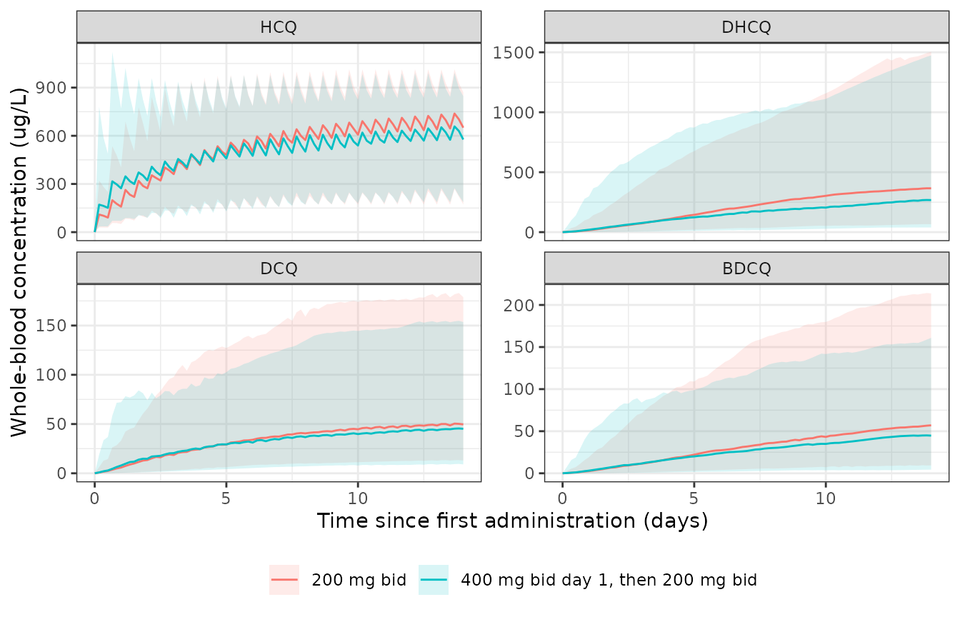
Simulated medians and 90% prediction intervals (without residual error); compare with the observed concentrations of Figure 2 of Alvarez 2022.
The Discussion describes the observed concentrations as roughly 500-1000 ug/L for hydroxychloroquine, around 500 ug/L for desethylhydroxychloroquine and 50-100 ug/L for desethylchloroquine and bisdesethylchloroquine, pooled over patients on different regimens and days. The typical-patient predictions on day 10 (just before the morning dose) for the two maintenance regimens are:
ev_typ10 <- dplyr::bind_rows(
  make_arm(1, data.frame(time = bid14, amt = 200), "200 mg bid"),
  make_arm(2, data.frame(time = seq(0, 328, by = 8), amt = 200), "200 mg tid")
) |>
  dplyr::arrange(id, time, dplyr::desc(evid))
day10 <- rxode2::rxSolve(mod_typ, events = ev_typ10, keep = "treatment") |>
  as.data.frame() |>
  dplyr::filter(time == 240) |>
  dplyr::select(treatment, dplyr::all_of(names(analytes))) |>
  tidyr::pivot_longer(dplyr::all_of(names(analytes)), names_to = "var", values_to = "conc") |>
  dplyr::mutate(analyte = unname(analytes[var]))
#> ℹ omega/sigma items treated as zero: 'etalcl', 'etalvc', 'etalcl_dhcq', 'etalcl_dcq', 'etalcl_bdcq'
#> Warning: multi-subject simulation without without 'omega'
stopifnot(nrow(day10) == 8L)
day10 |>
  dplyr::select(treatment, analyte, conc) |>
  tidyr::pivot_wider(names_from = analyte, values_from = conc) |>
  dplyr::rename("Regimen" = treatment) |>
knitr::kable(digits = 0, caption = "Typical-patient whole-blood concentrations (ug/L) on day 10.")| Regimen | HCQ | DHCQ | DCQ | BDCQ |
|---|---|---|---|---|
| 200 mg bid | 673 | 390 | 59 | 57 |
| 200 mg tid | 1034 | 580 | 89 | 85 |
c10 <- function(reg, a) {
  v <- day10$conc[day10$treatment == reg & day10$analyte == a]
  if (length(v) != 1L) stop("no unique day-10 row for ", reg, " / ", a)
  v
}
# Deterministic typical values. The Discussion's ranges are loose descriptions
# of pooled observations, so each is allowed a factor of 2 either way; a unit or
# molar-factor error, or a metabolite fed from the wrong compartment, moves a
# value by 8% to 1000-fold and the mass-balance gate above catches the small
# ones.
for (reg in c("200 mg bid", "200 mg tid")) {
  stopifnot(
    c10(reg, "HCQ") > 500 / 2, c10(reg, "HCQ") < 1000 * 2,
    c10(reg, "DHCQ") > 500 / 2, c10(reg, "DHCQ") < 500 * 2,
    c10(reg, "DCQ") > 50 / 2, c10(reg, "DCQ") < 100 * 2,
    c10(reg, "BDCQ") > 50 / 2, c10(reg, "BDCQ") < 100 * 2
  )
}
All four analytes fall inside the Discussion’s ranges for both regimens. The slower metabolites (desethylhydroxychloroquine and bisdesethylchloroquine, elimination half-lives of about 6 and 5 days) are still accumulating at day 10, as in Figure 2B.
Comparison against published NCA
The paper reports no non-compartmental parameters, so there is no published NCA table to compare with; the PKNCA analysis above is used for the mass-balance and half-life checks.
Assumptions and deviations
- Dose unit. Plaquenil 200 mg tablets contain 200 mg of hydroxychloroquine sulfate (about 155 mg of base). The fit used molar concentrations but does not say which molecular weight turned the dose into moles. Converting the labelled 200 mg with the free-base molecular weight reproduces the Figure 8 medians; treating it as sulfate salt (x 0.774 in moles) does not (Figure 8 section). The model therefore takes the labelled tablet strength in mg as the dose, and the apparent CL/F and VP/F are relative to that.
- Omega scale. Table 2 does not state whether the “omega” values are standard deviations or variances. They are entered as variances, following the same group’s lopinavir analysis; Figure 8 cannot separate the two readings (section above).
- Residual error. Proportional and additive terms are entered as standard deviations and combined in the nlmixr2 default (combined2) form; the paper states only “proportional plus additive”. The additive terms are used in the ug/L units printed in Table 2, although the fit itself was on umol/L.
- Metabolite volumes. Each metabolite volume equals the individual parent volume, including its eta, as the paper fixed VM/F to VP/F.
- Formation clearances carry no between-subject variability; Table 2 reports it only on CL/F, VP/F and the three metabolite elimination clearances.
- Molecular weights of the free bases (HCQ 335.87, DHCQ 307.82, DCQ 291.82, BDCQ 263.77 g/mol) come from their molecular formulas; the paper does not print them.
- Figure 4 panel labels. The first VPC panel is headed “DesOHCQ concentration” although the caption calls panel A hydroxychloroquine, and the second is headed “HCQ”; the figure panels, not the caption, were used for reading.
- Pharmacodynamic analysis not packaged. The length of stay was related to the model-predicted 48 h and 72 h troughs by linear regression (r^2 = 0.12 and 0.16) and clinical outcome by analysis of variance. These are statistical associations on the individual predictions, and the regression coefficients are not printed, so no PD model is included.