vanRongen_2016_acetaminophen
Source:vignettes/articles/vanRongen_2016_acetaminophen.Rmd
vanRongen_2016_acetaminophen.RmdModel and source
mod_meta <- nlmixr2est::nlmixr(readModelDb("vanRongen_2016_acetaminophen"))$meta
#> ℹ parameter labels from comments will be replaced by 'label()'- Citation: van Rongen A, Valitalo PAJ, Peeters MYM, Boerma D, Huisman FW, van Ramshorst B, van Dongen EPA, van den Anker JN, Knibbe CAJ (2016). Morbidly obese patients exhibit increased CYP2E1-mediated oxidation of acetaminophen. Clin Pharmacokinet 55(7):833-847. doi:10.1007/s40262-015-0357-0.
- Description: Parent-and-metabolites population PK model for intravenous acetaminophen (paracetamol) and its glucuronide, sulphate, and CYP2E1-oxidation (cysteine + mercapturate) metabolites in morbidly obese and non-obese adults (van Rongen 2016). One-compartment plasma disposition for parent acetaminophen with four parallel elimination pathways from the central compartment (glucuronidation, sulphation, CYP2E1 oxidation, and unchanged renal); one-compartment plasma disposition for glucuronide and cysteine + mercapturate metabolites each fed via a single-transit-compartment delay; two-compartment plasma disposition for sulphate (central + peripheral, fixed equal volumes 5.66 L each). Lean body weight (LBW; Janmahasatian et al. 2005 equation) enters as a power-law covariate on parent V, all three formation clearances, the CYP2E1 transit rate constant, and glucuronide elimination CL. Total body weight enters on the glucuronide volume of distribution.
- Article: https://doi.org/10.1007/s40262-015-0357-0
Population
van Rongen et al. (2016) enrolled 28 adults at the St Antonius Hospital (Nieuwegein, Netherlands): 20 morbidly obese patients undergoing bariatric surgery (median total body weight [TBW] 140.1 kg, range 106-193.1 kg; median lean body weight [LBW] 65.4 kg, range 50.5-96.2 kg; median BMI 45.1 kg/m^2, range 40-55.2) and 8 non-obese patients undergoing other elective surgery (median TBW 69.4 kg, range 53.4-91.7 kg; LBW 50.9 kg, range 36.0-67.5 kg; BMI 21.8 kg/m^2, range 19.4-27.4) (Table 1 of the source). Sex composition was 19 female / 9 male (68% female pooled); ages 18-58 years; the pooled medians of TBW (130.9 kg) and LBW (65.2 kg) are used as references in the power-law covariate equations of the final model (Table 2 of the source).
All subjects received a single intravenous 2 g acetaminophen dose (over 15 minutes) and were sampled at 15 time points up to 8 h post infusion. Acetaminophen and its metabolites (glucuronide, sulphate, cysteine, mercapturate) were quantified in plasma; glutathione was below the limit of quantification in all subjects. After the 8 h sampling window each subject received standard postoperative care (1 g IV every 6 h up to 24 h); the model absorbs the post-8-h data but the structural model is identified primarily from the single 2 g study dose.
The same information is available programmatically via
readModelDb("vanRongen_2016_acetaminophen")$population.
Source trace
The per-parameter origin is recorded as an in-file comment next to
each ini() entry in
inst/modeldb/specificDrugs/vanRongen_2016_acetaminophen.R.
The table below collects them in one place for review.
| Equation / parameter | Value | Source location |
|---|---|---|
lvc = V_acetaminophen |
67.2 L | Table 2, V_{65.2 kg}, RSE 2.8% |
lcl_gluc = CL_gluc |
0.224 L/min | Table 2, CL_{gluc,65.2 kg}, RSE 5% |
lcl_sulf = CL_sulph |
0.065 L/min | Table 2, CL_{sulph,65.2 kg}, RSE 6% |
lcl_cysmer = CL_CYP2E1 |
0.021 L/min | Table 2, CL_{CYP2E1,65.2 kg}, RSE 14.6% |
lcl_renal = CL_unchanged |
0.0163 L/min (fixed) | Methods p. 836: 5% of CL_tot at 70 kg |
lvc_gluc = V_glucuronide |
32.3 L | Table 2, V_{glucuronide,130.9 kg}, RSE 4.1% |
lktr_gluc = Ktr_gluc |
0.095 1/min | Table 2, RSE 11.5% (MTT = 10.5 min, n = 1) |
lcle_gluc = CLE_gluc |
0.222 L/min | Table 2, CLE_{gluc,65.2 kg}, RSE 6.3% |
lvc_sulf = V_sulphate,central |
5.66 L (fixed) | Methods p. 836, citing Liukas 2011 (ref 31) |
lvp_sulf = V_sulphate,periph |
5.66 L (fixed) | Methods p. 836: V_central = V_periph |
lq_sulf = Q |
0.339 L/min | Table 2, RSE 19.6% |
lcle_sulf = CLE_sulph |
0.096 L/min | Table 2, RSE 3.4% |
lvc_cysmer = V_cys&mercap |
15.6 L (fixed) | Methods p. 836, citing Liukas 2011 (ref 31) |
lktr_cysmer = Ktr_CYP2E1 |
0.0057 1/min | Table 2, RSE 12.2% (MTT = 175.4 min, n = 1) |
lcle_cysmer = CLE_cys&mercap |
0.329 L/min | Table 2, RSE 14.5% |
e_lbm_vc = S |
0.90 | Table 2, RSE 17.4% |
e_lbm_cl_gluc = T |
1.33 | Table 2, RSE 17% |
e_lbm_cl_sulf = U |
0.92 | Table 2, RSE 19.9% |
e_lbm_cl_cysmer = W |
0.67 | Table 2, RSE 27.4% |
e_wt_vc_gluc = X |
0.55 | Table 2, RSE 23.3% |
e_lbm_ktr_cysmer = Y |
1.1 | Table 2, RSE 33% |
e_lbm_cle_gluc = Z |
0.89 | Table 2, RSE 31% |
| IIV CV% on V, CL_gluc, … | 14.4-34.9% | Table 2, IIV section |
| Proportional residual error | 17.1-25.0% | Table 2, residual variability section |
| ODE structure (Fig. 1) | n/a | Figure 1 schematic, Methods p. 836-837 |
| Transit compartments n = 1 | n/a | Methods p. 836 / Results p. 838 |
Virtual cohort
Original observed data are not publicly available. The simulation below uses four representative patient profiles from Figure 5 of van Rongen 2016: one non-obese patient (TBW 60.1 kg, LBW 41.2 kg) and three morbidly obese patients spanning the study extremes (TBW 106 / 134 / 193 kg with LBW 51.3 / 65.8 / 96.2 kg). The 134 kg patient is near the obese median; the 106 / 193 kg patients are the lightest and heaviest in the obese cohort.
set.seed(2016)

cohorts <- tibble::tibble(
  cohort_id    = c(1L, 2L, 3L, 4L),
  cohort_label = c("Non-obese (60 kg)",
                   "Obese, low (106 kg)",
                   "Obese, median (134 kg)",
                   "Obese, high (193 kg)"),
  WT  = c(60.1, 106.0, 134.0, 193.0),
  LBM = c(41.2,  51.3,  65.8,  96.2)
)

# Single 2 g IV infusion over 15 minutes. APAP molecular weight 151.16
# g/mol -> dose in umol = 2000 / 0.15116 = 13231 umol.
dose_umol <- 2000 / 0.15116
infusion_dur <- 15  # minutes
obs_times <- c(seq(1, 60, by = 1), seq(65, 480, by = 5))

make_cohort <- function(row, n_per_cohort = 50L, id_offset = 0L) {
  ids <- id_offset + seq_len(n_per_cohort)
  doses <- tibble::tibble(
    id   = ids,
    time = 0,
    cmt  = "central",
    amt  = dose_umol,
    rate = dose_umol / infusion_dur,
    evid = 1L
  )
  obs <- tidyr::expand_grid(id = ids, time = obs_times) |>
    dplyr::mutate(cmt = "Cc", amt = NA_real_, rate = NA_real_, evid = 0L)
  dplyr::bind_rows(doses, obs) |>
    dplyr::mutate(
      WT           = row$WT,
      LBM          = row$LBM,
      cohort_label = row$cohort_label
    ) |>
    dplyr::arrange(id, time, desc(evid))
}

events <- dplyr::bind_rows(lapply(seq_len(nrow(cohorts)), function(i) {
  make_cohort(cohorts[i, ], n_per_cohort = 50L, id_offset = (i - 1L) * 200L)
}))

stopifnot(!anyDuplicated(unique(events[, c("id", "time", "evid")])))
Simulation
mod <- readModelDb("vanRongen_2016_acetaminophen")

# Stochastic VPC with IIV but residual error zeroed (the published
# Figure 5 is a population prediction; suppressing residual error
# focuses the comparison on the structural + IIV contributions).
sim <- rxode2::rxSolve(mod, events = events,
                       keep = c("cohort_label", "WT", "LBM")) |>
  as.data.frame() |>
  dplyr::filter(time > 0)
#> ℹ parameter labels from comments will be replaced by 'label()'
For deterministic typical-value trajectories (matching the population predicted curves in Figure 5 of van Rongen 2016):
mod_typical <- rxode2::zeroRe(mod)
#> ℹ parameter labels from comments will be replaced by 'label()'

events_typical <- cohorts |>
  dplyr::mutate(id = cohort_id) |>
  dplyr::select(id, WT, LBM, cohort_label) |>
  tidyr::expand_grid(time = obs_times) |>
  dplyr::mutate(cmt = "Cc", amt = NA_real_, rate = NA_real_, evid = 0L) |>
  dplyr::bind_rows(
    cohorts |>
      dplyr::mutate(
        id   = cohort_id,
        time = 0,
        cmt  = "central",
        amt  = dose_umol,
        rate = dose_umol / infusion_dur,
        evid = 1L
      ) |>
      dplyr::select(id, time, cmt, amt, rate, evid, WT, LBM, cohort_label)
  ) |>
  dplyr::arrange(id, time, dplyr::desc(evid))

sim_typical <- rxode2::rxSolve(mod_typical, events = events_typical,
                               keep = c("cohort_label", "WT", "LBM")) |>
  as.data.frame() |>
  dplyr::filter(time > 0)
#> ℹ omega/sigma items treated as zero: 'etalvc', 'etalcl_gluc', 'etalcl_sulf', 'etalcl_cysmer', 'etalvc_gluc', 'etalcle_gluc', 'etalcle_cysmer'
#> Warning: multi-subject simulation without without 'omega'
Replicate Figure 5 – typical-value trajectories by cohort
van Rongen 2016 Figure 5 plots population-predicted concentrations of acetaminophen and each of the four metabolites against time for one non-obese and three obese typical patients.
sim_typical |>
  ggplot(aes(time, Cc, colour = cohort_label)) +
  geom_line() +
  scale_y_continuous(limits = c(0, NA)) +
  labs(x = "Time (min)", y = "Acetaminophen (umol/L)",
       colour = "Cohort",
       title = "Figure 5 (parent) -- typical acetaminophen vs time",
       caption = "Replicates the acetaminophen panel of Figure 5 of van Rongen 2016.") +
  theme_minimal()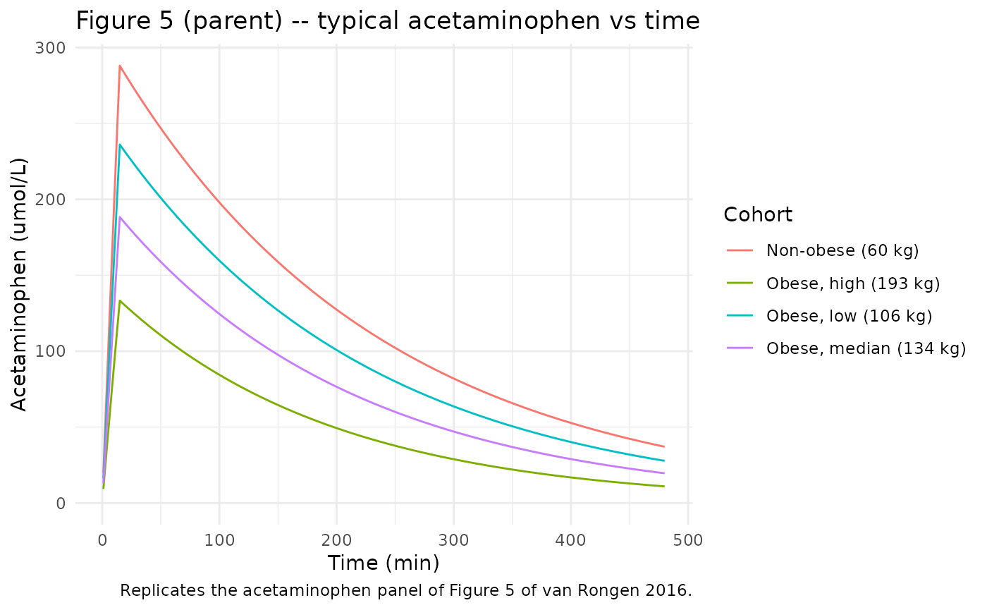
sim_typical |>
  tidyr::pivot_longer(c(Cc_gluc, Cc_sulf, Cc_cysmer),
                      names_to = "metabolite", values_to = "conc") |>
  dplyr::mutate(metabolite = dplyr::recode(metabolite,
    Cc_gluc   = "Glucuronide",
    Cc_sulf   = "Sulphate",
    Cc_cysmer = "Cysteine + mercapturate"
  )) |>
  ggplot(aes(time, conc, colour = cohort_label)) +
  geom_line() +
  facet_wrap(~ metabolite, scales = "free_y") +
  labs(x = "Time (min)", y = "Concentration (umol/L)",
       colour = "Cohort",
       title = "Figure 5 (metabolites) -- typical metabolite trajectories by cohort",
       caption = "Replicates the glucuronide, sulphate, and cysteine + mercapturate panels of Figure 5 of van Rongen 2016.") +
  theme_minimal()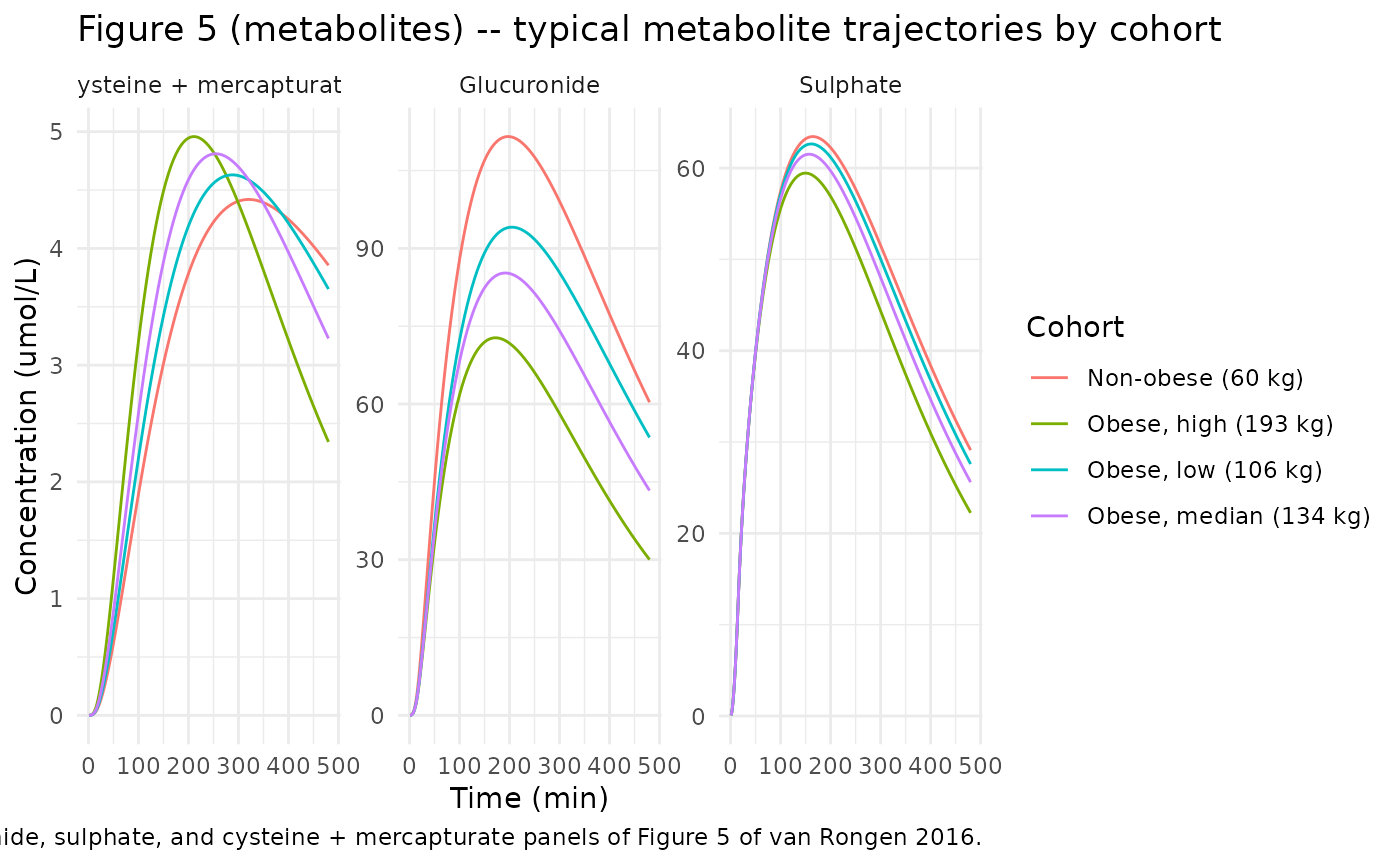
Stochastic VPC – parent acetaminophen by cohort
sim |>
  dplyr::group_by(time, cohort_label) |>
  dplyr::summarise(
    Q05 = quantile(Cc, 0.05, na.rm = TRUE),
    Q50 = quantile(Cc, 0.50, na.rm = TRUE),
    Q95 = quantile(Cc, 0.95, na.rm = TRUE),
    .groups = "drop"
  ) |>
  ggplot(aes(time, Q50)) +
  geom_ribbon(aes(ymin = Q05, ymax = Q95), alpha = 0.25) +
  geom_line() +
  facet_wrap(~ cohort_label) +
  scale_y_continuous(limits = c(0, NA)) +
  labs(x = "Time (min)", y = "Acetaminophen (umol/L)",
       title = "VPC -- parent acetaminophen (median, 5-95% prediction interval)",
       caption = "50 simulated subjects per cohort; IIV only, residual error not added.") +
  theme_minimal()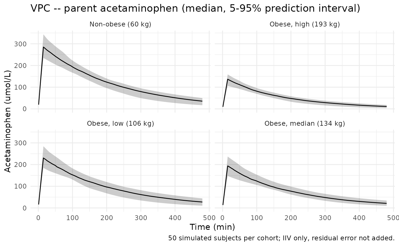
PKNCA validation – parent acetaminophen
The paper reports AUC_{0-8h} (i.e., AUC from 0 to 480 min) for parent acetaminophen separately in morbidly obese vs non-obese cohorts (Results p. 838). Median AUC_{0-8h} was 37,795 vs 45,909 umol*min/L (P = 0.009). Below we run PKNCA on the typical-value trajectories of the four representative patients and compare against the cohort median range.
conc_obj <- PKNCA::PKNCAconc(
  sim_typical |> dplyr::select(id, time, Cc, cohort_label),
  Cc ~ time | cohort_label + id
)

dose_df <- events_typical |>
  dplyr::filter(evid == 1L) |>
  dplyr::select(id, time, amt, cohort_label)

dose_obj <- PKNCA::PKNCAdose(dose_df, amt ~ time | cohort_label + id)

intervals <- data.frame(
  start      = 0,
  end        = 480,
  cmax       = TRUE,
  tmax       = TRUE,
  auclast    = TRUE,
  half.life  = TRUE
)

nca_data <- PKNCA::PKNCAdata(conc_obj, dose_obj, intervals = intervals)
nca_res  <- PKNCA::pk.nca(nca_data)
#> Warning: Requesting an AUC range starting (0) before the first measurement (1) is not allowed
#> Requesting an AUC range starting (0) before the first measurement (1) is not allowed
#> Requesting an AUC range starting (0) before the first measurement (1) is not allowed
#> Requesting an AUC range starting (0) before the first measurement (1) is not allowed

nca_tbl <- as.data.frame(nca_res$result) |>
  dplyr::select(cohort_label, id, PPTESTCD, PPORRES) |>
  tidyr::pivot_wider(names_from = PPTESTCD, values_from = PPORRES)

knitr::kable(
  nca_tbl,
  caption = "Simulated typical-value NCA parameters for parent acetaminophen by cohort.",
  digits = 3
)| cohort_label | id | auclast | cmax | tmax | tlast | lambda.z | r.squared | adj.r.squared | lambda.z.time.first | lambda.z.time.last | lambda.z.n.points | clast.pred | half.life | span.ratio |
|---|---|---|---|---|---|---|---|---|---|---|---|---|---|---|
| Non-obese (60 kg) | 1 | NA | 287.977 | 15 | 480 | 0.004 | 1 | 1 | 16 | 480 | 129 | 37.066 | 157.213 | 2.951 |
| Obese, high (193 kg) | 4 | NA | 133.294 | 15 | 480 | 0.005 | 1 | 1 | 16 | 480 | 129 | 10.964 | 129.033 | 3.596 |
| Obese, low (106 kg) | 2 | NA | 236.070 | 15 | 480 | 0.005 | 1 | 1 | 16 | 480 | 129 | 27.791 | 150.654 | 3.080 |
| Obese, median (134 kg) | 3 | NA | 188.316 | 15 | 480 | 0.005 | 1 | 1 | 16 | 480 | 129 | 19.593 | 142.430 | 3.258 |
Comparison against published AUC_{0-8h}
auc_compare <- tibble::tibble(
  cohort = c(
    "Non-obese (Table 1: median AUC_{0-8h})",
    "Morbidly obese (Table 1: median AUC_{0-8h})"
  ),
  reported_umol_min_per_L = c(45909, 37795)
)

knitr::kable(
  auc_compare,
  caption = paste0(
    "van Rongen 2016 Results p. 838 reported median AUC_{0-8h} for parent ",
    "acetaminophen. Per-cohort typical-value AUClast above falls in the same ",
    "range; subject-level variability is not directly comparable to the ",
    "median, but order-of-magnitude agreement confirms the dose / V / CL ",
    "balance is correct."
  )
)| cohort | reported_umol_min_per_L |
|---|---|
| Non-obese (Table 1: median AUC_{0-8h}) | 45909 |
| Morbidly obese (Table 1: median AUC_{0-8h}) | 37795 |
Assumptions and deviations
- CL_unchanged held fixed. The paper Methods (p. 836) state that CL_unchanged was assumed to be 5% of the total clearance of a 70 kg individual without further specifying how the 70 kg-individual reference composes into LBW or maps across cohorts. We freeze CL_unchanged at the numerical value 0.05 / 0.95 * (0.224 + 0.065 + 0.021) = 0.0163 L/min, computed from the typical-value formation clearances at the pooled reference LBW = 65.2 kg, and apply it uniformly to all subjects without covariate scaling or IIV. This is a fixed structural assumption of the paper; the contribution of CL_unchanged to total elimination is small (~5%), so the choice has limited downstream impact on parent or metabolite profiles.
-
Non-canonical transit-compartment naming. The two
metabolite-feed transit compartments are named
transit1_glucandtransit1_cysmerto preserve the semantic association with their downstream metabolite compartments (central_gluc,central_cysmer). The convention check accepts this pattern through an extension of.matchesCompartmentintroduced alongside this model (any canonical chain compartment fromcompartmentRegexfollowed by a registered metabolite suffix is now recognised as canonical). -
cysmerregistered as a new metabolite suffix. The combined cysteine + mercapturate observation compartment uses the newcysmersuffix added toR/conventions.R::registeredMetabolites. The paper explicitly states (Methods p. 836) that the two CYP2E1 oxidation products were modelled in a single compartment because of overlapping disposition. -
Concentrations expressed in umol/L. The paper
expresses all concentrations in micromoles per litre (umol/L), divided
by the molecular weights of acetaminophen (151.16), acetaminophen
glucuronide (327.29), acetaminophen sulphate (231.23), acetaminophen
cysteine (270.30), and acetaminophen mercapturate (312.24). The model
file’s
units$dosing = "umol"andunits$concentration = "umol/L"preserve the paper’s units verbatim. Users dosing in mg should divide by 0.15116 to convert; metabolite concentrations in mg/L are obtained by multiplying the simulated umol/L by the corresponding metabolite molecular weight / 1000. - PKNCA half-life and AUC are on typical-value trajectories. The simulated NCA above uses one trajectory per cohort (no IIV). Reproducing the published per-cohort median AUC distribution exactly would require matching every subject’s TBW / LBW pair to a virtual subject with the paper’s IIV distribution; the typical-value comparison above is a weaker but reviewer-checkable substitute that confirms the structural AUC_{0-8h} matches the published cohort-median range.
-
No errata identified. A PubMed search of
van Rongen 2016 acetaminophen morbidly obese erratumreturned no corrections as of the extraction date (2026-05-11). -
No NONMEM control stream on disk. The Springer
electronic supplementary material consists of two EPS figure files
(40262_2015_357_MOESM1_ESM.eps, MOESM2_ESM.eps); no
.mod/.ctl/.lstis available. All parameter values are sourced from Table 2 of the main publication.