Pneumocystis treatment QSP model (Liu 2018)
Source:vignettes/articles/Liu_2018_pneumocystis_qsp.Rmd
Liu_2018_pneumocystis_qsp.RmdModel and source
Liu 2018 builds three things and then composes them: a
three-compartment PK module, instantiated once per drug; a two-stage
Pneumocystis life-cycle PD module; and four integrated QSP
models, one per drug. The extraction mirrors that structure, so the
paper contributes five model files to
nlmixr2lib and this one vignette validates all of them.
qsp_models <- c(
  anidulafungin = "Liu_2018_anidulafungin_mouse_qsp",
  caspofungin = "Liu_2018_caspofungin_mouse_qsp",
  micafungin = "Liu_2018_micafungin_mouse_qsp",
  sulfamethoxazole = "Liu_2018_sulfamethoxazole_mouse_qsp"
)
pd_model <- "Liu_2018_pneumocystis_mouse_qsp"

# readModelDb() returns the model FUNCTION; rxode2::rxode() resolves it to the
# rxUi whose metadata fields are readable.
ui <- lapply(c(qsp_models, pneumocystis = pd_model), \(n) rxode2::rxode(readModelDb(n)))- Citation: Liu GS, Ballweg R, Ashbaugh A, Zhang Y, Facciolo J, Cushion MT, Zhang T. (2018). A quantitative systems pharmacology (QSP) model for Pneumocystis treatment in mice. BMC Syst Biol 12(1):77. doi:10.1186/s12918-018-0603-9. PK construction data (Liu 2018 Table 2 / reference 35) from Gumbo T, Drusano GL, Liu W, Ma L, Deziel MR, Drusano MF, Louie A. (2006). Anidulafungin pharmacokinetics and microbial response in neutropenic mice with disseminated candidiasis. Antimicrob Agents Chemother 50(11):3695-3700. doi:10.1128/AAC.00507-06. PK validation data (Liu 2018 Table 2 / reference 42) from Andes D, Diekema DJ, Pfaller MA, Prince RA, Marchillo K, Ashbeck J, Hou J. (2008). In vivo pharmacodynamic characterization of anidulafungin in a neutropenic murine candidiasis model. Antimicrob Agents Chemother 52(2):539-550. doi:10.1128/AAC.01061-07. Organism-burden data constraining the drug effect (Liu 2018 reference 33) from Cushion MT, Linke MJ, Ashbaugh A, Sesterhenn T, Collins MS, Lynch K, Brubaker R, Walzer PD. (2010). Echinocandin treatment of pneumocystis pneumonia in rodent models depletes cysts leaving trophic burdens that cannot transmit the infection. PLoS One 5(1):e8524. doi:10.1371/journal.pone.0008524.
- Article: https://doi.org/10.1186/s12918-018-0603-9
- PubMed Central: https://www.ncbi.nlm.nih.gov/pmc/articles/PMC6050661/
| Model | nlmixr2lib model | Role |
|---|---|---|
| anidulafungin | Liu_2018_anidulafungin_mouse_qsp | Integrated QSP: anidulafungin PK + Pneumocystis PD |
| caspofungin | Liu_2018_caspofungin_mouse_qsp | Integrated QSP: caspofungin PK + Pneumocystis PD |
| micafungin | Liu_2018_micafungin_mouse_qsp | Integrated QSP: micafungin PK + Pneumocystis PD |
| sulfamethoxazole | Liu_2018_sulfamethoxazole_mouse_qsp | Integrated QSP: sulfamethoxazole (TMP-SMX proxy) PK + Pneumocystis PD, with the 7-day effect delay |
| pneumocystis | Liu_2018_pneumocystis_mouse_qsp | PD module alone: untreated Pneumocystis natural history |
Population
The model was constrained with data from mice. Liu 2018’s own experiments used 6-week-old male C3H/HeN mice (Charles River) that were immunosuppressed and infected with Pneumocystis murina; organism burden was read out either by RT-qPCR of Pneumocystis mitochondrial large-subunit rRNA (total nuclei, which cannot distinguish the two life-cycle stages) or by microscopic quantification, using cresyl echt violet to stain asci specifically and a rapid Wright-Giemsa stain to count nuclei of all stages. The nuclei-count time course of Figure 3b has n = 2 or 3 mice per time point.
The PK modules were not fitted to new data. Liu 2018
digitised published murine plasma-concentration-versus-time figures with
labnotes and tuned each parameter set by hand:
anidulafungin from Gumbo 2006 (construction) and Andes 2008
(validation); caspofungin and micafungin from Andes 2010, with Hajdu
1997 as additional caspofungin validation; sulfamethoxazole from Misiek
1985. Organism burdens under treatment came from Cushion 2010, the
echinocandin depletion study that motivated the two-stage life-cycle
structure.
The TMP:SMX ratio was fixed at 1:5 in the constraining data, so Liu 2018 “used the level of SMX as a reasonable proxy for this drug combination” – the sulfamethoxazole model therefore carries a single drug, not two.
The same information is available programmatically:
str(ui[["anidulafungin"]]$population)
#> List of 9
#>  $ species       : chr "mouse (C3H/HeN)"
#>  $ n_subjects    : chr "PK module built on published murine plasma-concentration profiles digitised from Gumbo 2006 (construction) and "| __truncated__
#>  $ n_studies     : int 3
#>  $ age_range     : chr "6 weeks old at the start of the authors' own experiments"
#>  $ sex_female_pct: num 0
#>  $ disease_state : chr "Pneumocystis murina lung infection in immunosuppressed mice (the model of Pneumocystis pneumonia, PCP)"
#>  $ dose_range    : chr "0.1, 0.5, 1, 2.5, 5 and 10 mg/kg intraperitoneally (Liu 2018 Table 3); the Figure 4a treatment arms are 0.1, 0."| __truncated__
#>  $ regions       : chr "United States (University of Cincinnati; mice supplied by Charles River)"
#>  $ notes         : chr "Liu 2018 Experimental methods: 6-week-old male C3H/HeN mice. Organism burden quantified by RT-qPCR of Pneumocys"| __truncated__
Source trace
The per-parameter origin is recorded as an in-file comment next to
each ini() entry. The table below collects them in one
place.
| Equation / parameter | Value | Source location |
|---|---|---|
d/dt(depot) = -RAP*Kabs*depot |
n/a | Table 1 “Absorptive Compartment”; Methods equation (a) |
d/dt(central) = Kabs*depot - (KPT+KdP)*central + KTP*peripheral1 |
n/a | Table 1 “Plasma Compartment”; Methods equation (b) |
d/dt(peripheral1) = RTP*(-KTP*peripheral1 + KPT*central) - KdT*peripheral1 |
n/a | Table 1 “Peripheral Tissue Compartment”; Methods equation (c) |
lka (Kabs) |
5 / 5 / 0.75 / 5 per h | Table 1, row Kabs
|
lk12 (KPT) |
1.5 / 5 / 0.6 / 0.17 per h | Table 1, row KPT
|
lk21 (KTP) |
5 / 2 / 1.8 / 5 per h | Table 1, row KTP
|
lkel (KdP) |
0.035 / 0.18 / 0.06 / 0.2 per h | Table 1, row KdP
|
lkdt (KdT) |
0.035 / 0.18 / 0.06 / 0.2 per h | Table 1, row KdT
|
rap (RAP) |
3 / 0.1 / 1 / 3 | Table 1, row RAP
|
rtp (RTP) |
0.2 / 1 / 0.4 / 0.01 | Table 1, row RTP
|
| Initial AC concentration per dose | Table of 6 doses x 3 echinocandins | Table 3; SMX from the Table 3 footnote (“For SMX, 500 and 550 (ug/ml) were used for applied dosages of 200 and 250 (mg/kg) respectively”) |
d/dt(trophic) = KsTro*trophic - KdTro*trophic^2 - KTA*trophic + KAT*asci |
n/a | Table 4 “trophic Form”; Methods equation (d) |
d/dt(asci) = KTA*trophic - KAT*asci - KdAsci*asci |
n/a | Table 4 “asci”; Methods equation (e) |
kstro (KsTro) |
1 per day | Table 4, “Basal Parameter Values” |
kdtro (KdTro) |
1e-7 per day | Table 4, “Basal Parameter Values” |
kat (KAT) |
0.1 per day | Table 4, “Basal Parameter Values” |
kta (KTA) |
0.1 per day | Table 4, “Basal Parameter Values” |
kdasci (KdAsci) |
2e-12 per day | Table 4, “Basal Parameter Values” |
vdasci = kdAsci + ME*E/(E+Ec50) (echinocandin) |
n/a | Table 5, “Echinocandin effect on asci death” |
vta = kTA*(1 - E/(E+Ec50)) (echinocandin) |
n/a | Table 5, “Echinocandin effect on asci Formation” |
ec50, emax, hill
(echinocandin) |
0.039 / 0.0007 / 0.04 ug/mL; 0.42 / 0.45 / 0.1 per day; n = 1 | Table 5, echinocandin parameter table |
vdasci = kdAsci + MEAsci*E/(E+Ec50) (SMX) |
n/a | Table 5, “TMP/SMX effect on asci death” |
vstro = ks*(1 - E/(E+Ec50)) (SMX) |
n/a | Table 5, “TMP/SMX effect on trophic proliferation”; Methods |
vdtro = kdTro*(1 + METro*E/(E+Ec50)) (SMX) |
n/a | Table 5, “TMP/SMX effect on trophic death”; Methods |
smxeff = central(t - tau) |
n/a | Table 5, “Delay in SMX effect” |
ec50, hill, emax_asci,
emax_trophic, tau (SMX) |
0.2 ug/mL; n = 2; 0.75 per day; 650; 7 days | Table 5, TMP/SMX parameter table |
trophic0, asci0
|
1 organism each | Not reported. Back-solved from the paper’s described untreated time course; see “Assumptions and deviations” |
| PK-to-PD time-base conversion (x 24) | n/a | Derived: Table 1 is in 1/h, Table 4 in 1/day, Table 5’s tau in days |
| Dosing schedule | 3 doses/week for 3 weeks | Results, “Following the experimental dosing regimen reported by Cushion et al., each drug was elevated three times a week for 3 weeks” |
Part 1 – the PD module
Closed-form steady state (exact)
The drug-free system has an analytic non-trivial fixed point. Setting
d/dt(asci) = 0 gives
asci = KTA*trophic/(KAT + KdAsci); substituting into
d/dt(trophic) = 0 gives
trophic_ss = (KsTro - KTA + KAT*KTA/(KAT + KdAsci)) / KdTroBecause KdAsci is twelve orders of magnitude below
KAT, the two transformation terms cancel to working
precision and trophic_ss collapses to
KsTro / KdTro = 1 / 1e-7 = 1e7 – exactly the “steady state
of about 10^7” Liu 2018 reports. This is a deterministic identity, so it
is asserted tightly.
pd_par <- ui[["pneumocystis"]]$theta
tro_ss <- with(
  as.list(pd_par),
  (kstro - kta + kat * kta / (kat + kdasci)) / kdtro
)
asci_ss <- with(as.list(pd_par), kta * tro_ss / (kat + kdasci))

# Integrate far past equilibration and compare against the closed form.
ev_pd_long <- data.frame(
  id = 1L, time = seq(0, 400, by = 1),
  amt = NA_real_, evid = 0L, cmt = "trophic"
)
sim_pd_long <- rxode2::rxSolve(
  readModelDb(pd_model),
  events = ev_pd_long,
  atol = 1e-12, rtol = 1e-10,
  useLinCmt = FALSE
) |>
  as.data.frame()

tro_num <- tail(sim_pd_long$trophic, 1)
asci_num <- tail(sim_pd_long$asci, 1)

tibble::tibble(
  Quantity = c("trophic", "asci"),
  `Closed form` = c(tro_ss, asci_ss),
  `Numeric (day 400)` = c(tro_num, asci_num),
  `Relative difference` = c(abs(tro_num - tro_ss) / tro_ss, abs(asci_num - asci_ss) / asci_ss)
) |>
knitr::kable(digits = c(0, 0, 0, 12), caption = "Drug-free steady state: solver vs. closed form.")| Quantity | Closed form | Numeric (day 400) | Relative difference |
|---|---|---|---|
| trophic | 1e+07 | 1e+07 | 0 |
| asci | 1e+07 | 1e+07 | 0 |
Untreated accumulation (Figure 3b, and the pre-treatment phase of Figure 4c)
Liu 2018 describes the untreated time course in words: “The initial growth of the organism was very slow within the first two weeks, however, starting from the third week, an exponential growth of Pneumocystis was observed which peaked at the end of the fifth week”, and “At about 35 days, the levels of both trophic forms and asci reached a steady state of about 10^7”. Those three landmarks are what the day-0 inoculum was back-solved against (see “Assumptions and deviations”).
ev_pd <- data.frame(
  id = 1L, time = seq(0, 60, by = 0.25),
  amt = NA_real_, evid = 0L, cmt = "trophic"
)
sim_pd <- rxode2::rxSolve(
  readModelDb(pd_model),
  events = ev_pd,
  atol = 1e-12, rtol = 1e-10,
  useLinCmt = FALSE
) |>
  as.data.frame()

total_nuclei <- sim_pd$trophic + sim_pd$asci
sim_pd$normalised_total <- total_nuclei / max(total_nuclei)

sim_pd |>
  dplyr::select(time, trophic, asci) |>
  tidyr::pivot_longer(-time, names_to = "stage", values_to = "organisms") |>
  ggplot(aes(time, organisms, colour = stage)) +
  geom_line(linewidth = 0.9) +
  scale_y_log10(limits = c(1, 3e7)) +
  geom_vline(xintercept = 35, linetype = "dashed") +
  labs(
    x = "Time (day)", y = "Organisms per lung (log10 scale)",
    colour = "Life stage",
    title = "Untreated Pneumocystis accumulation",
    caption = paste(
      "Replicates the drug-free dynamics of Figure 3b and the pre-treatment",
      "phase of Figure 4c of Liu 2018. Dashed line: day 35."
    )
  )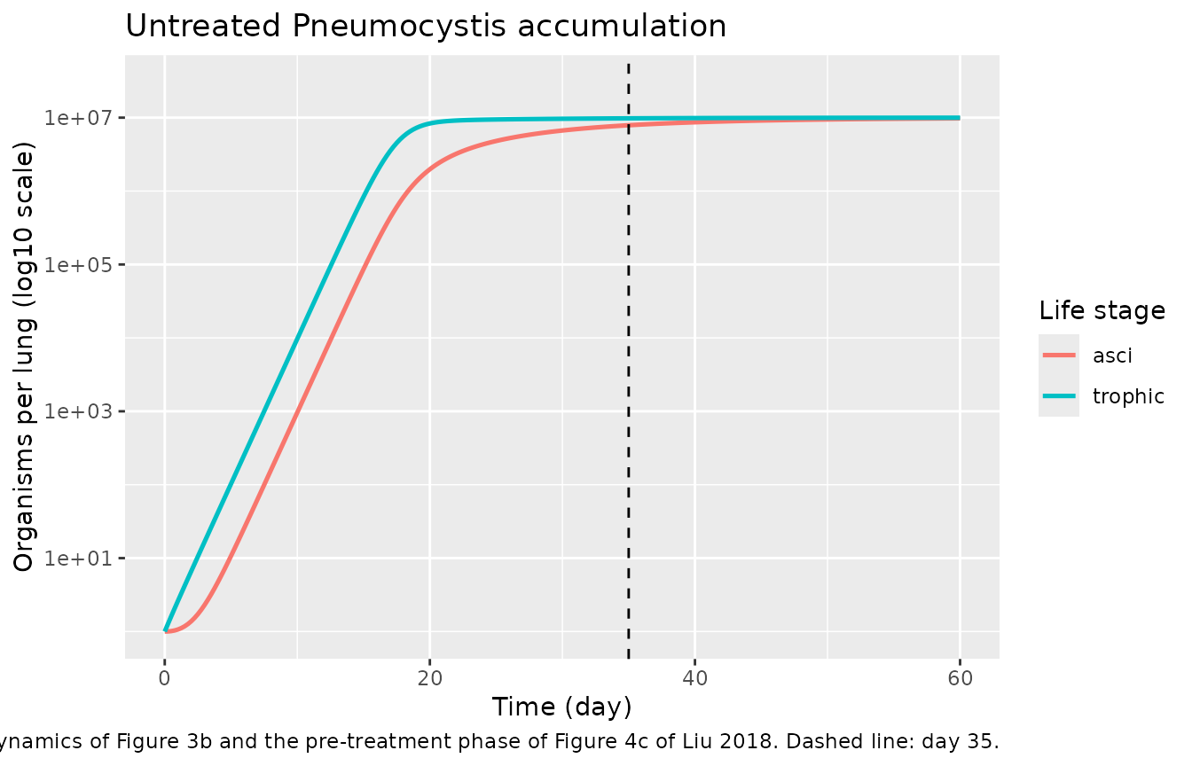
at <- function(d) sim_pd$normalised_total[which.min(abs(sim_pd$time - d))]
frac_35 <- sim_pd$trophic[which.min(abs(sim_pd$time - 35))] / tro_ss
t_half <- sim_pd$time[which(sim_pd$trophic >= 0.5 * tro_ss)[1]]

tibble::tibble(
  Landmark = c(
    "Normalised total nuclei at day 14 (paper: 'very slow' growth)",
    "Normalised total nuclei at day 21 (paper: exponential phase begins)",
    "Trophic burden at day 35 as a fraction of the plateau (paper: 'about 35 days ... steady state')",
    "Day at which the trophic burden crosses half the plateau"
  ),
  Value = c(at(14), at(21), frac_35, t_half)
) |>
knitr::kable(digits = 3, caption = "Figure 3b landmarks reproduced by the PD module.")| Landmark | Value |
|---|---|
| Normalised total nuclei at day 14 (paper: ‘very slow’ growth) | 0.020 |
| Normalised total nuclei at day 21 (paper: exponential phase begins) | 0.582 |
| Trophic burden at day 35 as a fraction of the plateau (paper: ‘about 35 days … steady state’) | 0.979 |
| Day at which the trophic burden crosses half the plateau | 17.750 |
# Deterministic run (no IIV in this model), so exact bounds are appropriate.
stopifnot(
  at(14) < 0.05, # still in the slow phase two weeks in
  at(21) > at(14), # exponential growth has started by week three
  frac_35 > 0.95, # plateau essentially reached by day 35
  t_half > 14, t_half < 25 # the rise is centred in weeks three and four
)
Asci repopulation after echinocandin withdrawal (Figure 3a)
Figure 3a starts “from an initial state with a high level of trophic forms and a low level of asci” and shows that “it takes several weeks for asci to repopulate”. Rather than invent that initial state, it is taken from the anidulafungin QSP model’s own day-56 output (built in Part 3 below) and the drug-free PD module is then integrated forward.
dose_days <- c(35, 37, 39, 42, 44, 46, 49, 51, 53)

make_qsp_events <- function(ac0, dose_days, tmax = 56, by = 0.25) {
  obs <- data.frame(
    id = 1L, time = seq(0, tmax, by = by),
    amt = NA_real_, evid = 0L, cmt = "trophic"
  )
  if (is.null(ac0)) {
    return(obs[order(obs$time), ])
  }
  dose <- data.frame(
    id = 1L, time = dose_days, amt = ac0, evid = 1L, cmt = "depot"
  )
  out <- dplyr::bind_rows(dose, obs)
  out[order(out$time, -out$evid), ]
}

solve_qsp <- function(model, events) {
  rxode2::rxSolve(
    readModelDb(model),
    events = events,
    atol = 1e-12, rtol = 1e-10, maxsteps = 1e6,
    useLinCmt = FALSE
  ) |>
    as.data.frame()
}

# Anidulafungin 1 mg/kg i.p. => initial AC concentration 10 ug/mL (Table 3).
sim_anid <- solve_qsp(qsp_models[["anidulafungin"]], make_qsp_events(10, dose_days))
post_treatment <- c(
  trophic = tail(sim_anid$trophic, 1),
  asci = tail(sim_anid$asci, 1)
)

ev_recover <- data.frame(
  id = 1L, time = seq(0, 90, by = 0.25),
  amt = NA_real_, evid = 0L, cmt = "trophic"
)
sim_recover <- rxode2::rxSolve(
  readModelDb(pd_model),
  events = ev_recover,
  inits = post_treatment,
  atol = 1e-12, rtol = 1e-10,
  useLinCmt = FALSE
) |>
  as.data.frame()

sim_recover |>
  dplyr::select(time, trophic, asci) |>
  tidyr::pivot_longer(-time, names_to = "stage", values_to = "organisms") |>
  ggplot(aes(time, organisms, colour = stage)) +
  geom_line(linewidth = 0.9) +
  scale_y_log10() +
  labs(
    x = "Days after withdrawal of anidulafungin", y = "Organisms per lung (log10 scale)",
    colour = "Life stage",
    title = "Asci repopulate over several weeks once the echinocandin stops",
    caption = "Replicates Figure 3a of Liu 2018."
  )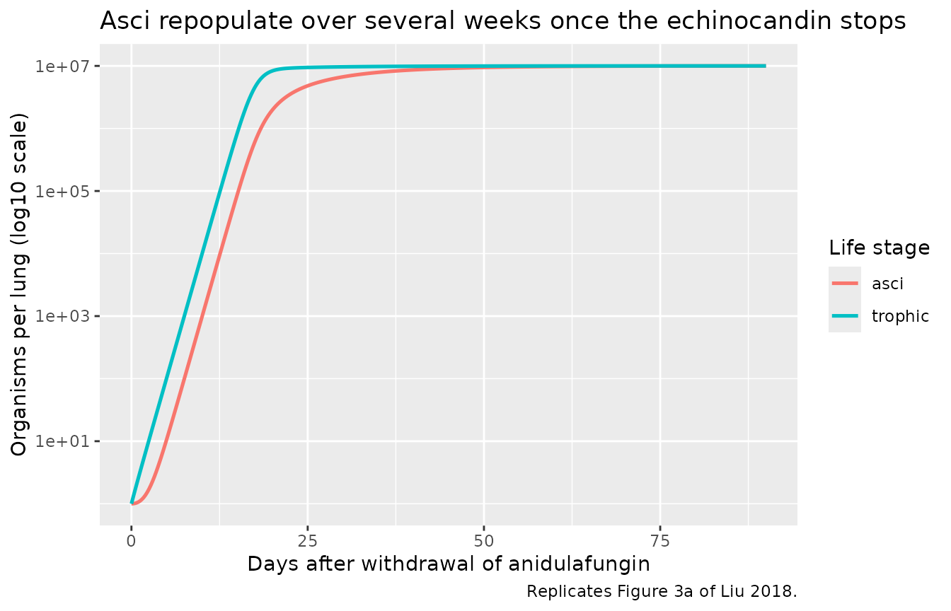
# Time for the asci to recover to within 0.3 log10 of their drug-free plateau.
t_recover <- sim_recover$time[which(sim_recover$asci >= 10^(log10(asci_ss) - 0.3))[1]]
cat(sprintf(
  "Asci start %.2f log10 below the drug-free plateau and recover to within 0.3 log10 of it after %.1f days (%.1f weeks).\n",
  log10(asci_ss) - log10(post_treatment[["asci"]]), t_recover, t_recover / 7
))
#> Asci start 1.65 log10 below the drug-free plateau and recover to within 0.3 log10 of it after 25.5 days (3.6 weeks).
# The paper's claim is qualitative -- "several weeks". Bracket it loosely
# enough to be a real test of the KTA / KAT timescale and no tighter.
stopifnot(t_recover > 7, t_recover < 70)
Population of PD models (Figures 3c and 3d)
“To recapture these experimentally observed distributions, we constructed a population of PD models with parameter values selected from a uniform distribution that covers 70-130% of the basal values (Table 4). … In order to incorporate variability, all model parameters are changed independently.”
The five PD rate constants are therefore resampled independently on
U(0.7 x basal, 1.3 x basal). These draws come from R’s RNG,
not rxode2’s, so the cohort is reproducible across machines and thread
counts.
set.seed(20260918)
n_pop <- 200L # cohort cap is 200 per arm
pd_names <- c("kstro", "kdtro", "kta", "kat", "kdasci")
basal <- pd_par[pd_names]

pop <- as.data.frame(lapply(basal, \(b) runif(n_pop, 0.7 * b, 1.3 * b)))
pop$trophic0 <- pd_par[["trophic0"]]
pop$asci0 <- pd_par[["asci0"]]
pop$id <- seq_len(n_pop)

ev_pop <- tidyr::expand_grid(id = pop$id, time = c(0, 60)) |>
  dplyr::mutate(amt = NA_real_, evid = 0L, cmt = "trophic") |>
  as.data.frame()

sim_pop <- rxode2::rxSolve(
  readModelDb(pd_model),
  params = pop,
  events = ev_pop,
  atol = 1e-12, rtol = 1e-10,
  useLinCmt = FALSE
) |>
  as.data.frame() |>
  dplyr::filter(time == 60)

sim_pop |>
  dplyr::select(id, log10_trophic, log10_asci) |>
  tidyr::pivot_longer(-id, names_to = "stage", values_to = "log10_organisms") |>
  dplyr::mutate(stage = dplyr::recode(stage,
    log10_trophic = "trophic form",
    log10_asci = "asci"
  )) |>
  ggplot(aes(log10_organisms)) +
  geom_histogram(bins = 25) +
  facet_wrap(~stage) +
  labs(
    x = "log10 organisms per lung at day 60", y = "Simulated mice",
    title = "Simulated burden distributions under 70-130% parameter resampling",
    caption = "Replicates Figures 3c and 3d of Liu 2018."
  )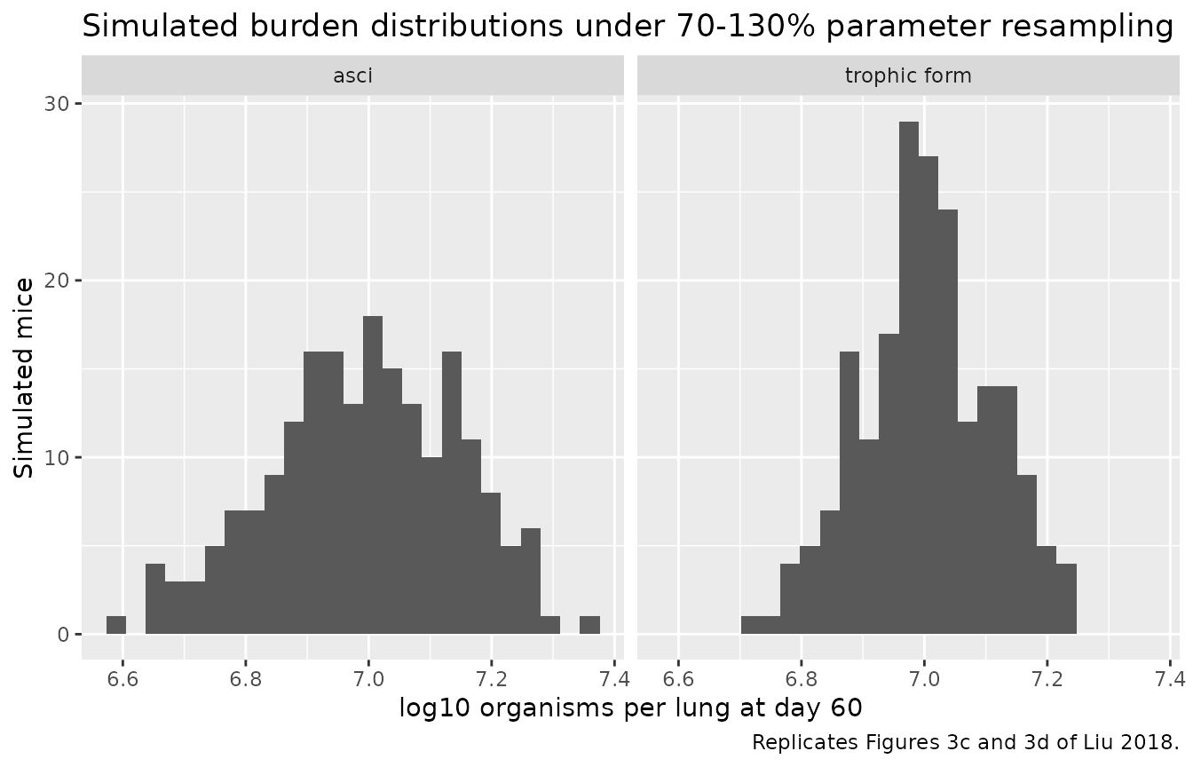
# Liu 2018 Results: 'the simulated distributions of the trophic forms (Fig. 3c)
# and asci (Fig. 3d) are consistent to the observed levels of the fungi
# (7.62 +/- 0.17 for trophic forms and 7.79 +/- 0.13 for asci) [33]'.
burden_summary <- tibble::tibble(
  Stage = c("trophic form", "asci"),
  `Simulated median (log10)` = c(median(sim_pop$log10_trophic), median(sim_pop$log10_asci)),
  `Simulated range (log10)` = c(
    sprintf("%.2f - %.2f", min(sim_pop$log10_trophic), max(sim_pop$log10_trophic)),
    sprintf("%.2f - %.2f", min(sim_pop$log10_asci), max(sim_pop$log10_asci))
  ),
  `Observed, Cushion 2010 (log10)` = c("7.62 +/- 0.17", "7.79 +/- 0.13")
)
knitr::kable(burden_summary, digits = 2, caption = "Simulated vs. observed steady-state burdens.")| Stage | Simulated median (log10) | Simulated range (log10) | Observed, Cushion 2010 (log10) |
|---|---|---|---|
| trophic form | 7 | 6.73 - 7.23 | 7.62 +/- 0.17 |
| asci | 7 | 6.59 - 7.36 | 7.79 +/- 0.13 |
# The simulated plateau is KsTro / KdTro exactly, so a 70-130% resample can
# reach at most log10(1.3 / (0.7e-7)) = 7.27. The observed means of 7.62 and
# 7.79 therefore sit ABOVE anything this parameterisation can produce -- a
# reproducible deviation from the paper's consistency claim, recorded under
# 'Assumptions and deviations' rather than papered over. What is asserted here
# is the arithmetic the model does commit to.
stopifnot(
  # Centre of the resampled distribution is the basal plateau, log10(1e7) = 7.
  abs(median(sim_pop$log10_trophic) - 7) < 0.15,
  # And every draw lies inside the algebraic envelope of the resampling.
  all(sim_pop$log10_trophic >= log10(0.7 / 1.3e-7) - 0.01),
  all(sim_pop$log10_trophic <= log10(1.3 / 0.7e-7) + 0.01)
)
Part 2 – the PK module
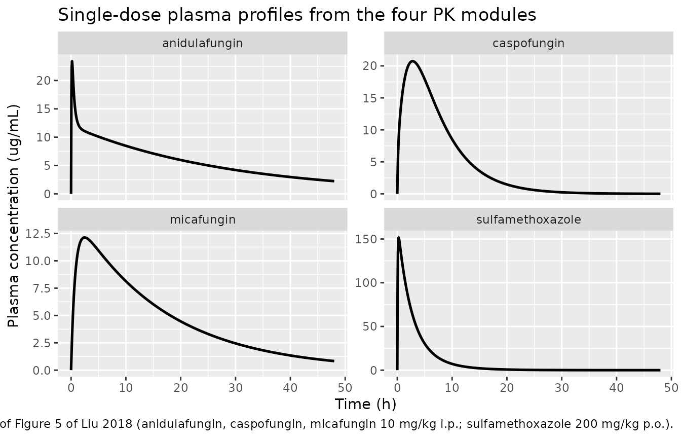
Closed-form plasma AUC (exact)
Integrating the three PK equations from zero to infinity turns them into three linear algebraic equations in the three areas. Solving them gives an exact plasma AUC for any dose placed in the administration compartment:
AUC_plasma = (AC0 / RAP) / ( (KPT + KdP) - KPT*KTP*RTP / (RTP*KTP + KdT) )Both scaling factors appear where the paper’s asymmetric structure
puts them: RAP divides the administered concentration (only
a fraction 1/RAP of it reaches plasma) and RTP
enters the tissue-recirculation term only. This is an algebraic
identity, so agreement with the solver should be at machine precision –
which makes it a sharp check that the ODEs were transcribed correctly,
including the asymmetries.
# Table 3 row 1: the highest tabulated i.p. dose per echinocandin, and the
# 200 mg/kg oral sulfamethoxazole dose from the Table 3 footnote.
ac0_single <- c(
  anidulafungin = 90, # 10 mg/kg i.p.
  caspofungin = 12, # 10 mg/kg i.p.
  micafungin = 25, # 10 mg/kg i.p.
  sulfamethoxazole = 500 # 200 mg/kg p.o.
)

auc_closed <- function(model) {
  p <- as.list(rxode2::rxode(readModelDb(model))$theta)
  ka <- exp(p$lka)
  k12 <- exp(p$lk12)
  k21 <- exp(p$lk21)
  kel <- exp(p$lkel)
  kdt <- exp(p$lkdt)
  1 / ((k12 + kel) - k12 * k21 * p$rtp / (p$rtp * k21 + kdt)) / p$rap
}

# Single i.p. / p.o. dose, observed on a fine grid over 10 days. Observation
# rows sit on the `central` ODE state so that the algebraic observable Cc is
# returned at every one of them.
make_pk_events <- function(ac0, tmax = 10, n = 4001L) {
  dose <- data.frame(id = 1L, time = 0, amt = ac0, evid = 1L, cmt = "depot")
  obs <- data.frame(
    id = 1L, time = seq(0, tmax, length.out = n),
    amt = NA_real_, evid = 0L, cmt = "central"
  )
  out <- dplyr::bind_rows(dose, obs)
  out[order(out$time, -out$evid), ]
}

sim_pk <- lapply(names(qsp_models), function(d) {
  s <- solve_qsp(qsp_models[[d]], make_pk_events(ac0_single[[d]]))
  s$drug <- d
  # rxSolve omits `id` for a single-subject event table.
  s$id <- 1L
  s
}) |>
  dplyr::bind_rows() |>
  # Report time in hours: Table 1 is in 1/h and Figure 5 is plotted in hours.
  dplyr::mutate(time_h = time * 24)
#> [====|====|====|====|====|====|====|====|====|====] 0:00:00

stopifnot(all(sim_pk$Cc >= 0))
sim_pk |>
  dplyr::filter(time_h <= 48) |>
  ggplot(aes(time_h, Cc)) +
  geom_line(linewidth = 0.9) +
  facet_wrap(~drug, scales = "free_y") +
  labs(
    x = "Time (h)", y = "Plasma concentration (ug/mL)",
    title = "Single-dose plasma profiles from the four PK modules",
    caption = paste(
      "Replicates the black construction curves of Figure 5 of Liu 2018",
      "(anidulafungin, caspofungin, micafungin 10 mg/kg i.p.;",
      "sulfamethoxazole 200 mg/kg p.o.)."
    )
  )
The module also reproduces the paper’s i.v.-versus-i.p. contrast
(Figure 5a, blue): “in order to mimic i.v. injection, we elevated the
initial level of the drug in the plasma compartment”, which is a dose
into central rather than depot. The two routes
share the same disposition parameters, so an i.v. dose of
AC0/RAP must give the same plasma AUC as an i.p. dose of
AC0 – another exact consequence of the structure.
ev_iv <- dplyr::bind_rows(
  data.frame(id = 1L, time = 0, amt = 90 / 3, evid = 1L, cmt = "central"),
  data.frame(
    id = 1L, time = seq(0, 10, length.out = 4001L),
    amt = NA_real_, evid = 0L, cmt = "central"
  )
)
ev_iv <- ev_iv[order(ev_iv$time, -ev_iv$evid), ]
sim_iv <- solve_qsp(qsp_models[["anidulafungin"]], ev_iv)

dplyr::bind_rows(
  dplyr::mutate(sim_iv, route = "i.v. 30 ug/mL into plasma"),
  dplyr::mutate(
    dplyr::filter(sim_pk, drug == "anidulafungin"),
    route = "i.p. 90 ug/mL into the AC"
  )
) |>
  dplyr::filter(time * 24 <= 36) |>
  ggplot(aes(time * 24, Cc, colour = route)) +
  geom_line(linewidth = 0.9) +
  labs(
    x = "Time (h)", y = "Plasma anidulafungin (ug/mL)", colour = NULL,
    title = "Anidulafungin: i.v. versus i.p. administration",
    caption = "Replicates the route contrast of Figure 5a of Liu 2018."
  ) +
  theme(legend.position = "bottom")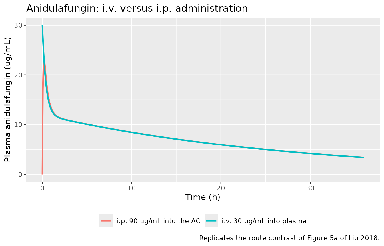
PKNCA on the simulated plasma profiles
Liu 2018 reports no NCA table – it reports SSE against digitised profiles instead, and argues in the Discussion that the temporal predictions are more informative than “traditional pharmacokinetic indexes such as area under the curve”. The NCA below is therefore not a comparison against published NCA values; it exists to turn the exact AUC identity above into an independent, tool-computed check of the same quantity, and to put interpretable Cmax / Tmax / half-life numbers on each module.
# Only `!is.na(Cc)` -- filtering on time or Cc would drop the time-zero row
# that PKNCA needs to anchor AUC.
sim_nca <- sim_pk |>
  dplyr::filter(!is.na(Cc)) |>
  dplyr::select(id, time = time_h, Cc, drug)

sim_nca <- dplyr::bind_rows(
  sim_nca,
  sim_nca |> dplyr::distinct(id, drug) |> dplyr::mutate(time = 0, Cc = 0)
) |>
  dplyr::distinct(id, drug, time, .keep_all = TRUE) |>
  dplyr::arrange(drug, id, time)

conc_obj <- PKNCA::PKNCAconc(as.data.frame(sim_nca), Cc ~ time | drug + id)

dose_df <- sim_pk |>
  dplyr::distinct(drug, id) |>
  dplyr::mutate(time = 0, amt = ac0_single[drug]) |>
  as.data.frame()
dose_obj <- PKNCA::PKNCAdose(dose_df, amt ~ time | drug + id)

intervals <- data.frame(
  start = 0, end = Inf,
  cmax = TRUE, tmax = TRUE, aucinf.obs = TRUE, half.life = TRUE
)

nca_res <- PKNCA::pk.nca(PKNCA::PKNCAdata(conc_obj, dose_obj, intervals = intervals))
nca_wide <- as.data.frame(nca_res) |>
  dplyr::select(drug, PPTESTCD, PPORRES) |>
  tidyr::pivot_wider(names_from = PPTESTCD, values_from = PPORRES)

nca_wide$auc_closed <- vapply(
  nca_wide$drug,
  \(d) auc_closed(qsp_models[[d]]) * ac0_single[[d]],
  numeric(1)
)
nca_wide$auc_pct_diff <- 100 * (nca_wide$aucinf.obs - nca_wide$auc_closed) / nca_wide$auc_closed

nca_wide |>
  dplyr::select(drug, cmax, tmax, half.life, aucinf.obs, auc_closed, auc_pct_diff) |>
  dplyr::rename(
    "Drug" = drug,
    "Cmax (ug/mL)" = cmax,
    "Tmax (h)" = tmax,
    "t1/2 (h)" = half.life,
    "PKNCA AUCinf (ug*h/mL)" = aucinf.obs,
    "Closed-form AUC (ug*h/mL)" = auc_closed,
    "Difference (%)" = auc_pct_diff
  ) |>
  knitr::kable(
    digits = c(0, 2, 2, 2, 1, 1, 4),
    caption = paste(
      "PKNCA parameters of the four PK modules after a single dose, with",
      "AUCinf checked against the closed-form identity."
    )
)| Drug | Cmax (ug/mL) | Tmax (h) | t1/2 (h) | PKNCA AUCinf (ug*h/mL) | Closed-form AUC (ug*h/mL) | Difference (%) |
|---|---|---|---|---|---|---|
| anidulafungin | 23.41 | 0.18 | 19.78 | 349.8 | 350.0 | -0.0388 |
| caspofungin | 20.73 | 2.82 | 3.85 | 202.4 | 202.4 | -0.0093 |
| micafungin | 12.13 | 2.46 | 11.55 | 235.5 | 235.5 | -0.0025 |
| sulfamethoxazole | 151.72 | 0.24 | 3.45 | 495.3 | 496.0 | -0.1522 |
# Deterministic models and an algebraic target: the agreement is numerical
# error only, so the bound is tight. A transcription error in any of ka, k12,
# k21, kel, kdt, rap or rtp moves this by whole percent or more.
stopifnot(
  nrow(nca_wide) == 4L,
  all(!is.na(nca_wide$aucinf.obs)),
  max(abs(nca_wide$auc_pct_diff)) < 0.5
)
Multiple dosing three times a week (Figure 6)
mw_days <- c(0, 2, 4, 7, 9, 11, 14, 16, 18)
echino_doses <- list(
  anidulafungin = c(`10 mg/kg` = 90, `1 mg/kg` = 10, `0.1 mg/kg` = 1),
  caspofungin = c(`10 mg/kg` = 12, `1 mg/kg` = 2.5, `0.1 mg/kg` = 0.8),
  micafungin = c(`10 mg/kg` = 25, `1 mg/kg` = 5, `0.1 mg/kg` = 1)
)

sim_fig6 <- lapply(names(echino_doses), function(d) {
  lapply(names(echino_doses[[d]]), function(lv) {
    ev <- make_qsp_events(echino_doses[[d]][[lv]], mw_days, tmax = 21, by = 0.02)
    s <- solve_qsp(qsp_models[[d]], ev)
    s$drug <- d
    s$dose <- lv
    s
  }) |> dplyr::bind_rows()
}) |>
  dplyr::bind_rows()

sim_fig6 |>
  dplyr::filter(time <= 7) |>
  ggplot(aes(time, Cc, colour = dose)) +
  geom_line(linewidth = 0.7) +
  facet_wrap(~drug, scales = "free_y") +
  labs(
    x = "Time (day)", y = "Plasma concentration (ug/mL)", colour = "Dose",
    title = "Echinocandin plasma levels over one week of 3-doses-per-week treatment",
    caption = "Replicates panels a-c of Figure 6 of Liu 2018 (first week shown)."
  ) +
  theme(legend.position = "bottom")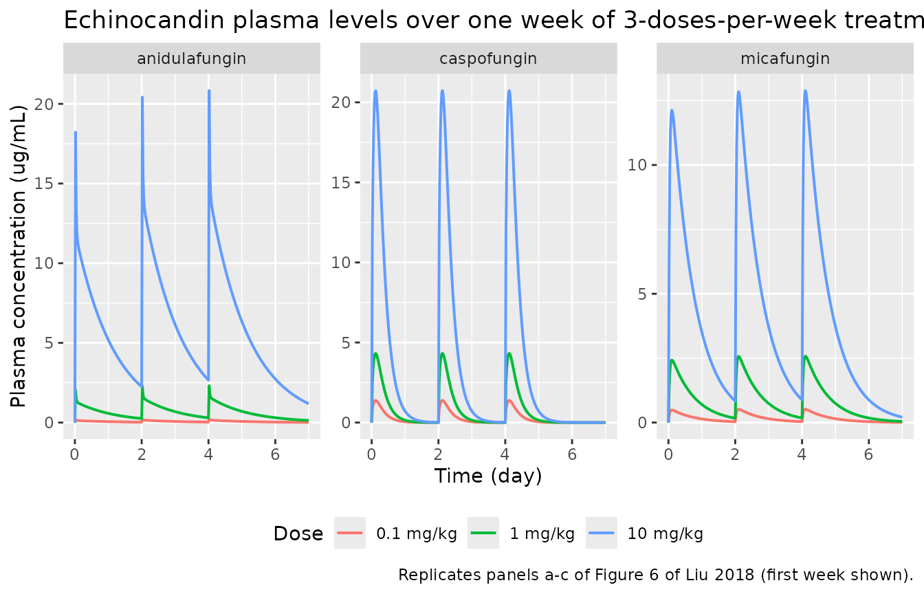
ev_smx3w <- make_qsp_events(500, mw_days, tmax = 21, by = 0.02)
sim_smx3w <- solve_qsp(qsp_models[["sulfamethoxazole"]], ev_smx3w)

ggplot(sim_smx3w, aes(time, Cc)) +
  geom_line(linewidth = 0.7) +
  labs(
    x = "Time (day)", y = "Plasma sulfamethoxazole (ug/mL)",
    title = "Sulfamethoxazole 200 mg/kg orally, 3 doses per week for 3 weeks",
    caption = "Replicates panel d of Figure 6 of Liu 2018."
  )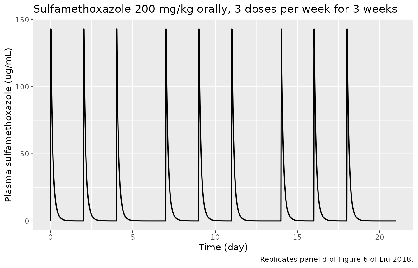
# Liu 2018 shows no drug accumulation across the 3-doses-per-week schedule: the
# echinocandin half-lives are hours and the inter-dose interval is 2-3 days, so
# each peak should repeat rather than climb. Deterministic, so assert exactly.
peaks <- sim_fig6 |>
  dplyr::filter(dose == "10 mg/kg") |>
  dplyr::mutate(week = findInterval(time, c(0, 7, 14))) |>
  dplyr::group_by(drug, week) |>
  dplyr::summarise(peak = max(Cc), .groups = "drop") |>
  tidyr::pivot_wider(names_from = week, values_from = peak, names_prefix = "week")

knitr::kable(peaks, digits = 3, caption = "Peak echinocandin concentration in each treatment week (10 mg/kg).")| drug | week1 | week2 | week3 |
|---|---|---|---|
| anidulafungin | 20.833 | 20.873 | 20.874 |
| caspofungin | 20.733 | 20.733 | 20.733 |
| micafungin | 12.888 | 12.889 | 12.889 |
Part 3 – the integrated QSP models
Treatment starts once the infection has plateaued. Liu 2018 gives each drug “3 times per week for 3 weeks” and reads out “the simulated levels of asci at day 56”; the pre-treatment plateau is reached “at about 35 days”, and 35 + 21 = 56, so the treatment window is days 35 to 56 on a Monday / Wednesday / Friday schedule.
Day-56 burden by drug and dose (Figures 4a and 4b)
arms <- tibble::tribble(
  ~drug, ~dose_label, ~ac0,
  "anidulafungin", "1 mg/kg", 10,
  "anidulafungin", "0.5 mg/kg", 5,
  "anidulafungin", "0.1 mg/kg", 1,
  "caspofungin", "1 mg/kg", 2.5,
  "caspofungin", "0.5 mg/kg", 1.5,
  "caspofungin", "0.1 mg/kg", 0.8,
  "micafungin", "1 mg/kg", 5,
  "micafungin", "0.5 mg/kg", 3,
  "micafungin", "0.1 mg/kg", 1,
  "sulfamethoxazole", "200 mg/kg", 500
)

sim_arms <- Map(
  function(d, lab, a) {
    s <- solve_qsp(qsp_models[[d]], make_qsp_events(a, dose_days))
    s$drug <- d
    s$dose_label <- lab
    s
  },
  arms$drug, arms$dose_label, arms$ac0
) |>
  dplyr::bind_rows()

sim_control <- solve_qsp(qsp_models[["anidulafungin"]], make_qsp_events(NULL, dose_days))
control_56 <- c(
  trophic = tail(sim_control$log10_trophic, 1),
  asci = tail(sim_control$log10_asci, 1)
)

day56 <- sim_arms |>
  dplyr::filter(time == 56) |>
  dplyr::transmute(
    drug, dose_label,
    log10_asci, log10_trophic,
    asci_reduction = control_56[["asci"]] - log10_asci,
    trophic_reduction = control_56[["trophic"]] - log10_trophic
  )

dplyr::bind_rows(
  tibble::tibble(
    drug = "control (untreated)", dose_label = "-",
    log10_asci = control_56[["asci"]], log10_trophic = control_56[["trophic"]],
    asci_reduction = 0, trophic_reduction = 0
  ),
  day56
) |>
  dplyr::rename(
    "Drug" = drug,
    "Dose" = dose_label,
    "log10 asci" = log10_asci,
    "log10 trophic" = log10_trophic,
    "Asci reduction (log10)" = asci_reduction,
    "Trophic reduction (log10)" = trophic_reduction
  ) |>
  knitr::kable(
    digits = 2,
    caption = "Day-56 Pneumocystis burden. Replicates Figures 4a and 4b of Liu 2018."
)| Drug | Dose | log10 asci | log10 trophic | Asci reduction (log10) | Trophic reduction (log10) |
|---|---|---|---|---|---|
| control (untreated) | - | 6.99 | 7.00 | 0.00 | 0.00 |
| anidulafungin | 1 mg/kg | 5.35 | 6.99 | 1.64 | 0.00 |
| anidulafungin | 0.5 mg/kg | 5.62 | 6.99 | 1.37 | 0.01 |
| anidulafungin | 0.1 mg/kg | 6.16 | 6.98 | 0.83 | 0.02 |
| caspofungin | 1 mg/kg | 5.86 | 6.98 | 1.12 | 0.02 |
| caspofungin | 0.5 mg/kg | 5.93 | 6.98 | 1.06 | 0.02 |
| caspofungin | 0.1 mg/kg | 6.00 | 6.98 | 0.98 | 0.02 |
| micafungin | 1 mg/kg | 5.93 | 6.99 | 1.06 | 0.01 |
| micafungin | 0.5 mg/kg | 6.07 | 6.99 | 0.91 | 0.01 |
| micafungin | 0.1 mg/kg | 6.36 | 6.98 | 0.62 | 0.01 |
| sulfamethoxazole | 200 mg/kg | 4.42 | 4.86 | 2.57 | 2.14 |
dplyr::bind_rows(
  tibble::tibble(
    drug = "control", dose_label = "-",
    log10_asci = control_56[["asci"]], log10_trophic = control_56[["trophic"]]
  ),
  dplyr::select(day56, drug, dose_label, log10_asci, log10_trophic)
) |>
  tidyr::pivot_longer(c(log10_asci, log10_trophic), names_to = "stage", values_to = "log10_organisms") |>
  dplyr::mutate(
    stage = dplyr::recode(stage, log10_asci = "asci (Fig. 4a)", log10_trophic = "trophic form (Fig. 4b)"),
    arm = paste(drug, dose_label)
  ) |>
  ggplot(aes(reorder(arm, log10_organisms), log10_organisms)) +
  geom_col() +
  facet_wrap(~stage) +
  coord_flip() +
  labs(
    x = NULL, y = "log10 organisms per lung at day 56",
    title = "Day-56 burden by treatment arm",
    caption = "Replicates Figures 4a and 4b of Liu 2018."
  )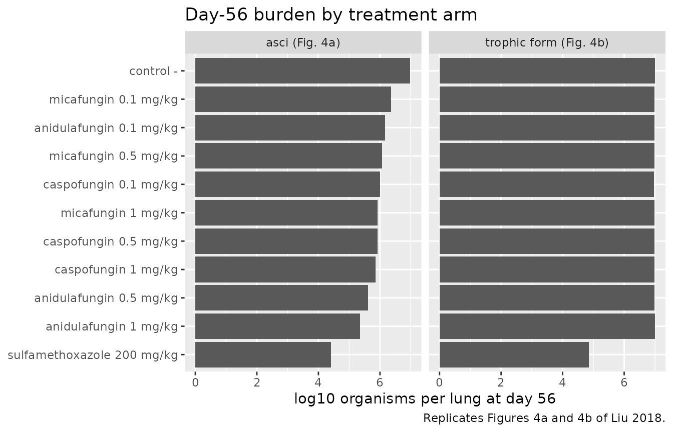
The paper’s qualitative claims about this figure are checked
mechanically. Every quantity below is a deterministic output of a model
with no random effects and a solver run at atol = 1e-12 /
rtol = 1e-10 (results are unchanged across observation
grids of 0.5, 0.25 and 0.05 days), so exact orderings and tight bounds
are legitimate here in a way they would not be for a simulated
cohort.
One claim is not reproduced and is marked as such rather than having its bound widened until it passes: see the narrative below the table.
red <- function(d, lab, what) {
  v <- day56[[paste0(what, "_reduction")]][day56$drug == d & day56$dose_label == lab]
  if (length(v) != 1L) stop("no unique row for ", d, " ", lab)
  v
}
asci_red <- function(d, lab) red(d, lab, "asci")

min_1mg <- min(
  asci_red("anidulafungin", "1 mg/kg"),
  asci_red("caspofungin", "1 mg/kg"),
  asci_red("micafungin", "1 mg/kg")
)
max_troph <- max(day56$trophic_reduction[day56$drug != "sulfamethoxazole"])
# Margin by which micafungin is the weakest of the three, at each dose.
mica_margin <- vapply(
  c("1 mg/kg", "0.5 mg/kg", "0.1 mg/kg"),
  \(lab) {
    min(asci_red("anidulafungin", lab), asci_red("caspofungin", lab)) -
      asci_red("micafungin", lab)
  },
  numeric(1)
)
smx_min <- min(
  asci_red("sulfamethoxazole", "200 mg/kg"),
  red("sulfamethoxazole", "200 mg/kg", "trophic")
)

claims <- tibble::tribble(
  ~Claim, ~Quantity, ~Achieved, ~Pass, ~Deviation,
  "At 1 mg/kg all three echinocandins 'considerably reduced asci burdens'",
  "minimum asci reduction across the three drugs at 1 mg/kg (log10)",
  min_1mg, min_1mg > 0.9, FALSE,

  "'the simulated trophic forms were not meaningfully altered following treatment with any of the echinocandins'",
  "maximum trophic reduction across all nine echinocandin arms (log10)",
  max_troph, max_troph < 0.05, FALSE,

  "Micafungin is the weakest of the three echinocandins at every tested dose (the ordering behind the Figure 4a claim)",
  "smallest margin, across the three doses, by which micafungin is out-reduced by both other drugs (log10)",
  min(mica_margin), min(mica_margin) > 0.03, FALSE,

  "'micafungin caused no notable decrease in the levels of asci' at 0.5 and 0.1 mg/kg",
  "micafungin asci reduction at 0.1 mg/kg (log10); 'no notable decrease' read as under 0.3",
  asci_red("micafungin", "0.1 mg/kg"), asci_red("micafungin", "0.1 mg/kg") < 0.3, TRUE,

  "'The model showed a marked decrease in both asci and trophic forms in response to TMP/SMX treatment'",
  "minimum of the TMP/SMX asci and trophic reductions (log10)",
  smx_min, smx_min > 1.5, FALSE
)

claims |>
  dplyr::mutate(Pass = ifelse(Deviation, paste0(Pass, " (deviation)"), as.character(Pass))) |>
  dplyr::select(-Deviation) |>
knitr::kable(digits = 3, caption = "Liu 2018 Figure 4a / 4b claims, checked against the packaged models.")| Claim | Quantity | Achieved | Pass |
|---|---|---|---|
| At 1 mg/kg all three echinocandins ‘considerably reduced asci burdens’ | minimum asci reduction across the three drugs at 1 mg/kg (log10) | 1.060 | TRUE |
| ‘the simulated trophic forms were not meaningfully altered following treatment with any of the echinocandins’ | maximum trophic reduction across all nine echinocandin arms (log10) | 0.023 | TRUE |
| Micafungin is the weakest of the three echinocandins at every tested dose (the ordering behind the Figure 4a claim) | smallest margin, across the three doses, by which micafungin is out-reduced by both other drugs (log10) | 0.063 | TRUE |
| ‘micafungin caused no notable decrease in the levels of asci’ at 0.5 and 0.1 mg/kg | micafungin asci reduction at 0.1 mg/kg (log10); ‘no notable decrease’ read as under 0.3 | 0.622 | FALSE (deviation) |
| ‘The model showed a marked decrease in both asci and trophic forms in response to TMP/SMX treatment’ | minimum of the TMP/SMX asci and trophic reductions (log10) | 2.139 | TRUE |
# Gate on everything except the row recorded as a known deviation.
stopifnot(all(claims$Pass[!claims$Deviation]))
The one row marked as a deviation is the literal reading of
“micafungin caused no notable decrease in the levels of asci”. The
reconstructed model does put micafungin last at every dose – that
ordering is reproduced, and it is what distinguishes micafungin’s
ME = 0.1 /day from anidulafungin’s 0.42 and
caspofungin’s 0.45 – but it still predicts a 0.62 log10
asci reduction at 0.1 mg/kg, which is not “no notable decrease”. Figure
4a plots the simulations against experimental dot plots with standard
errors, so a 0.6 log10 shift may well be inside the experimental scatter
the authors were judging against; no parameter was changed to close the
gap.
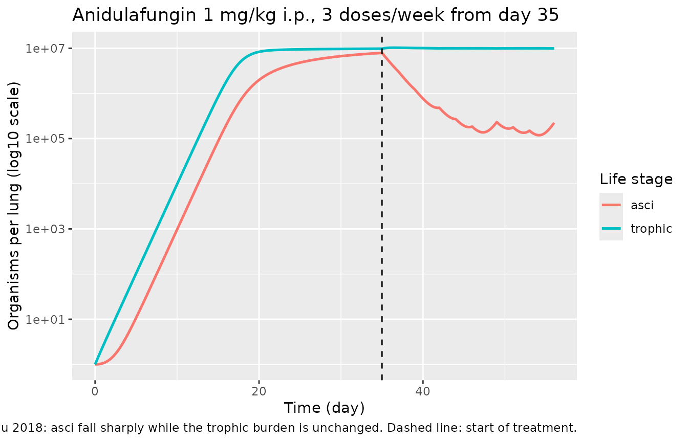
Anidulafungin time course (Figure 4c)
sim_anid |>
  dplyr::select(time, trophic, asci) |>
  tidyr::pivot_longer(-time, names_to = "stage", values_to = "organisms") |>
  ggplot(aes(time, organisms, colour = stage)) +
  geom_line(linewidth = 0.9) +
  scale_y_log10() +
  geom_vline(xintercept = 35, linetype = "dashed") +
  labs(
    x = "Time (day)", y = "Organisms per lung (log10 scale)", colour = "Life stage",
    title = "Anidulafungin 1 mg/kg i.p., 3 doses/week from day 35",
    caption = paste(
      "Replicates Figure 4c of Liu 2018: asci fall sharply while the trophic",
      "burden is unchanged. Dashed line: start of treatment."
    )
  )
TMP/SMX time course and the seven-day effect delay (Figure 4d)
The sulfamethoxazole model is the only one of the four that is a
genuine delay differential equation: the effect is driven by
central(t - 7 days), encoded with
rxode2::delay(). Liu 2018 introduced the delay because “in
comparison with the rapid antifungal effect of anidulafungin, the
experimental evidence suggests that the effect of TMP-SMX was
delayed”.
sim_smx <- solve_qsp(qsp_models[["sulfamethoxazole"]], make_qsp_events(500, dose_days))

sim_smx |>
  dplyr::select(time, trophic, asci) |>
  tidyr::pivot_longer(-time, names_to = "stage", values_to = "organisms") |>
  ggplot(aes(time, organisms, colour = stage)) +
  geom_line(linewidth = 0.9) +
  scale_y_log10() +
  geom_vline(xintercept = c(35, 42), linetype = c("dashed", "dotted")) +
  labs(
    x = "Time (day)", y = "Organisms per lung (log10 scale)", colour = "Life stage",
    title = "TMP/SMX 200 mg/kg orally, 3 doses/week from day 35",
    caption = paste(
      "Replicates Figure 4d of Liu 2018. Dashed line: first dose (day 35).",
      "Dotted line: day 42, when the 7-day-delayed effect can first appear."
    )
  )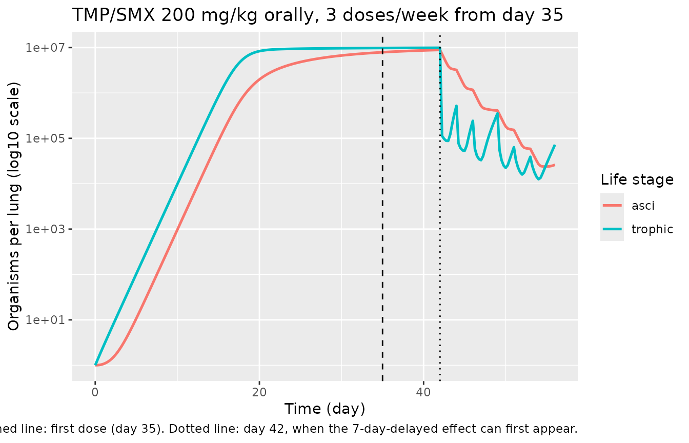
# The delay is a hard structural feature: before day 35 + tau the delayed
# plasma level is still the pre-dose value of zero, so NO effect is possible.
tau <- ui[["sulfamethoxazole"]]$theta[["tau"]]
before <- sim_smx |> dplyr::filter(time > 35, time < 35 + tau)
after <- sim_smx |> dplyr::filter(time >= 35 + tau)

drop_before <- max(before$log10_trophic) - min(before$log10_trophic)
drop_after <- max(before$log10_trophic) - min(after$log10_trophic)

tibble::tibble(
  Window = c(
    sprintf("day 35 to day %.0f (inside the delay)", 35 + tau),
    sprintf("day %.0f to day 56 (delay elapsed)", 35 + tau)
  ),
  `Trophic swing (log10)` = c(drop_before, drop_after)
) |>
knitr::kable(digits = 3, caption = "The seven-day delay gates the onset of the TMP/SMX effect.")| Window | Trophic swing (log10) |
|---|---|
| day 35 to day 42 (inside the delay) | 0.004 |
| day 42 to day 56 (delay elapsed) | 2.896 |
Assumptions and deviations
-
Day-0 organism inoculum is not reported. Liu 2018
tabulates initial drug concentrations (Table 3) but nowhere states the
day-0 Pneumocystis burden that Figures 3b and 4c start from.
trophic0andasci0are therefore back-solved, not transcribed: the drug-free system’s linearised net growth rate is 0.910/day, and a unit inoculum of each stage is the value that reproduces all three landmarks the paper does state in prose – growth “very slow within the first two weeks”, exponential “starting from the third week”, and a plateau of “about 10^7” reached “at about 35 days”. Both are exposed asini()parameters so any other infection scenario can be simulated by overriding them or by passinginits =torxSolve(). This is the only non-paper-derived value in the five model files. -
PK-to-PD time-base conversion. Table 1 reports the
PK rate constants in 1/h while Table 4 reports the PD rate constants in
1/day and Table 5’s delay in days. Liu 2018 does not say which base the
integrated model ran on. The models put everything on a
day base – the QSP readouts are at day 35 and day 56 –
by multiplying the whole (entirely first-order) PK right-hand side by
24. The
ini()values remain the Table 1 numbers verbatim, insidelog(). Running the PK module on an hour base instead would leave the PK identical and scale every PD rate by 1/24; that the day base reproduces the Figure 4a dose ranking, including micafungin’s lack of effect at 0.1 mg/kg, is evidence it is the base the authors used. -
No IIV and no residual error. Liu 2018 reports
neither an omega nor a sigma; it is a deterministic model tuned by hand
(“all parameters sets and initial conditions were derived manually using
a trial and error method”). No etas and no residual-error terms were
invented. Every parameter is wrapped in
fixed()to record that it was held, not estimated. Variability in the paper is generated instead by resampling the five PD rate constants onU(70%, 130%)of their basal values, which the Figure 3c / 3d chunk above reproduces explicitly. -
The simulated burden distribution sits about 0.6 log10 below
the observed levels the paper compares it with. Liu 2018 states
that the Figure 3c / 3d distributions “are consistent to the observed
levels of the fungi (7.62 +/- 0.17 for trophic forms and 7.79 +/- 0.13
for asci)”. With the Table 4 values the trophic plateau is exactly
KsTro / KdTro = 1 / 1e-7 = 1e7, i.e. log10 7.00, and a 70-130% independent resample can reach at most log10(1.3 / 0.7e-7) = 7.27. The observed means of 7.62 and 7.79 are therefore above anything this parameterisation can produce. This is arithmetic, not a simulation artefact, and it is recorded here rather than worked around: no parameter was altered to close the gap, and the assertion in that chunk tests the algebra the model does commit to (the plateau is the basalKsTro / KdTroand every draw lies inside the resampling envelope). -
Micafungin’s “no notable decrease” at low dose is not
reproduced literally. Liu 2018 reads Figure 4a as showing that
at 0.5 and 0.1 mg/kg “anidulafungin and caspofungin still decreased the
number of asci, while micafungin caused no notable decrease”. The
packaged models reproduce the ordering – micafungin is the
weakest of the three at every tested dose, which is what its
ME = 0.1 /dayversus 0.42 and 0.45 buys – but predict a 0.62 log10 asci reduction for micafungin at 0.1 mg/kg, which is not literally “no notable decrease”. Figure 4a compares simulations against experimental dot plots with standard errors, so a shift of that size may sit inside the scatter the authors were judging against. The claim is carried in the Figure 4a / 4b claims table as an explicit deviation row and excluded from that chunk’s assertion; nothing was retuned to close it. - Monday / Wednesday / Friday dosing schedule. Liu 2018 says only “three times a week for 3 weeks” following Cushion 2010, without printing the calendar. Days 35, 37, 39, 42, 44, 46, 49, 51 and 53 are used (a M/W/F pattern for three weeks starting at the day-35 plateau), giving nine doses and a day-56 readout, which matches the paper’s own 35 + 21 = 56 arithmetic and its “levels of asci at day 56”.
- No published NCA table to compare against. The paper reports goodness of fit as SSE against digitised concentration-time profiles (Table 2: 459.26, 2602.56, 202.14 and 131.15 for anidulafungin, caspofungin, micafungin and SMX) and argues in the Discussion that temporal predictions are more informative than “single indices such as steady state AUC”. The PKNCA section therefore validates the PK modules against an exact closed-form AUC identity derived from the paper’s own equations rather than against transcribed NCA values, and reports Cmax / Tmax / half-life for orientation. The SSE values are not reproducible here because the digitised construction and validation datasets are not published.
-
Non-mass-conserving PK structure reproduced
verbatim.
RAPmultiplies the loss term of the administration compartment but not the matching gain term in plasma, andRTPmultiplies both transfer terms of the tissue equation but neither of the plasma equation. The equations are transcribed as printed rather than “corrected” into a mass-balanced system; the closed-form AUC check above is derived from the same asymmetric equations and agrees with the solver to better than 0.5%, so the asymmetries are intentional and self-consistent, not a transcription error. - A mis-citation in the paper’s own prose. Methods states that “the initial level of Anidulafungin was estimated to be 90 ug/ml for the i.p. dosage of 10 mg/kg (34)”, but reference 34 is Cushion 2006, a bisbenzamidine efficacy study with no anidulafungin PK. Table 3 attributes the same 90 ug/mL to reference 35 (Gumbo 2006), which is the anidulafungin PK source named in Table 2. The model files cite Gumbo 2006; the “(34)” in the prose is an unlinked typographical slip.
-
useLinCmt = FALSEon every solve. These models carryk12/k21peripheral transfer alongside non-PK ODE states. rxode2’s default automatic ODE-to-linCmt()conversion mishandles that shape, so everyrxSolve()call in this vignette passesuseLinCmt = FALSE.