Mycophenolic acid (Dong 2014)
Source:vignettes/articles/Dong_2014_mycophenolic_acid.Rmd
Dong_2014_mycophenolic_acid.RmdModel and source
- Citation: Dong M, Fukuda T, Cox S, de Vries MT, Hooper DK, Goebel J, Vinks AA. Population pharmacokinetic-pharmacodynamic modelling of mycophenolic acid in paediatric renal transplant recipients in the early post-transplant period. Br J Clin Pharmacol. 2014;78(5):1102-1112. doi:10.1111/bcp.12426.
- Description: Population PK-PD model for oral mycophenolic acid (MPA, the active moiety of mycophenolate mofetil MMF) in paediatric renal transplant recipients in the early post-transplant period (Dong 2014). Two-compartment disposition with a Savic 2007-style 8-transit-compartment absorption chain followed by a first-order absorption step from depot to central; dose-dependent relative bioavailability described by a power function of dose per body surface area (DBSA) with reference 450 mg/m^2; estimated body-weight exponent of 0.31 on CL/F (not the canonical allometric 0.75). The PD layer links MPA plasma concentration to inosine monophosphate dehydrogenase (IMPDH) activity in peripheral blood mononuclear cells via a simplified inhibitory Emax model with Emax fixed at 0 (i.e., complete inhibition achievable in the limit of high MPA concentration).
- Article: https://doi.org/10.1111/bcp.12426
Population
The Dong 2014 model is a single-site population PK-PD analysis of oral mycophenolic acid (MPA, the active moiety of mycophenolate mofetil MMF) in 24 paediatric kidney transplant recipients followed during the early post-transplant period (days 4-9 post-transplantation) at Cincinnati Children’s Hospital Medical Center. The PK cohort had a median (range) age of 14.2 (2.1-20.2) years, median weight 38.2 (10.3-106.4) kg, median BSA 1.26 (0.49-2.21) m^2, 37.5% female, and 83% Caucasian / 17% African American. All patients were on tacrolimus + prednisone backbone immunosuppression with basiliximab or rabbit antithymocyte globulin (Thymoglobulin) induction; patients on cyclosporine were excluded. A subset of 17 patients with 97 IMPDH activity measurements in peripheral blood mononuclear cells contributed to the PK-PD fit. See Dong 2014 Table 1 for the per-cohort baseline demographics.
The same information is available programmatically via
rxode2::rxode(readModelDb("Dong_2014_mycophenolic_acid"))$population.
Source trace
The per-parameter origin is recorded as a trailing in-file comment
next to each ini() entry in
inst/modeldb/specificDrugs/Dong_2014_mycophenolic_acid.R.
The table below collects them in one place.
| Equation / parameter | Value | Source location (Dong 2014) |
|---|---|---|
lcl (CL/F at 70 kg) |
22.0 L/h | Table 2 row “CL/F (L/h/70 kg)” theta1 |
lvc (Vc/F) |
45.4 L | Table 2 row “Vc/F (L)” |
lvp (Vp/F) |
411 L | Table 2 row “Vp/F (L)” |
lq (Q/F) |
22.4 L/h | Table 2 row “Q/F (L/h)” |
lka (ka) |
2.5 1/h | Table 2 row “Ka (h-1)” |
lmtt (MTT) |
0.25 h | Table 2 row “MTT (h)” |
lnn (n_transit) |
8 (FIXED) | Table 2 row “Number of transit compartment (n)” |
e_wt_cl (WT exponent on CL) |
0.31 | Table 2 row “theta2” (estimated, not 0.75) |
e_dbsa_f (DBSA exponent on F) |
-0.43 | Table 2 row “theta4” (theta3 fixed at 1) |
lrbase (E0, IMPDH baseline) |
3.45 nmol/h/mg | Table 3 row “E0 (nmol h-1 mg-1 protein)” |
lec50 (EC50) |
1.73 mg/L | Table 3 row “EC50 (mg/L)” |
| Emax (asymptotic minimum activity) | 0 (FIXED) | Table 3 row “Emax (nmol h-1 mg-1 protein) = 0 fix” |
etalcl |
log(1 + 0.259^2) = 0.0649 | Table 2 omega(CL/F) = 25.9% CV |
etalka |
log(1 + 2.996^2) = 2.300 | Table 2 omega(Ka) = 299.6% CV |
etalmtt |
log(1 + 1.448^2) = 1.130 | Table 2 omega(MTT) = 144.8% CV |
etalrbase |
log(1 + 0.396^2) = 0.1459 | Table 3 omega(E0) = 39.6% CV |
etalec50 |
log(1 + 0.725^2) = 0.4226 | Table 3 omega(EC50) = 72.5% CV |
expSd (PK residual SD, log scale) |
0.51 | Table 2 footnote c: %CV = 51.0; sigma = 0.51^2 = 0.2601 |
propSd_impdh (PD proportional SD) |
0.422 | Table 3 footnote c: %CV = 42.2; sigma = 0.422^2 = 0.1781 |
| Transit chain ODE | n/a | Equation 6 (Savic & Karlsson 2007 with Stirling approximation) |
| Bioavailability power function | n/a | Equation 5 |
| Inhibitory Emax PD | n/a | Equation 7 (with Emax fixed at 0) |
Virtual cohort
The original individual-level data are not publicly available. The simulation below uses a 60-subject virtual paediatric cohort whose body weight distribution approximates Dong 2014 Table 1 and whose body surface area is derived from weight via the Mosteller formula assuming a weight-band-appropriate height (a simple monotonic height-weight approximation; the source paper does not state which BSA formula it used). Each subject receives a starting dose of either 450 or 600 mg/m^2 MMF twice daily, matching the two institutional starting protocols described in Methods.
set.seed(2014)

n_subj <- 60

# Sample body weight to approximate the cohort weight distribution
# (Dong 2014 Table 1: median 38.2 kg, range 10.3-106.4 kg). Log-uniform on
# [10, 100] kg gives a flat representation across the paediatric range so
# the AUC vs DBSA replication exercises the full weight span.
wt_kg <- exp(runif(n_subj, log(10), log(100)))

# Approximate height from weight using a simple monotonic relationship
# anchored at the paediatric percentiles (10 kg ~ 75 cm; 40 kg ~ 140 cm;
# 70 kg ~ 168 cm). Used only to compute BSA via Mosteller; not a covariate
# in the model.
ht_cm <- 45 + 110 * (wt_kg / 70) ^ 0.45

# Body surface area via Mosteller (BSA m^2 = sqrt(WT_kg * HT_cm / 3600)).
bsa_m2 <- sqrt(wt_kg * ht_cm / 3600)

# Each subject is randomised to one of the two starting MMF protocols
# (450 or 600 mg/m^2 BID); the per-subject dose in mg is the protocol value
# times BSA, rounded to the nearest 50 mg as in routine prescribing.
protocol_mg_m2 <- sample(c(450, 600), n_subj, replace = TRUE)
dose_mg_per_event <- round(protocol_mg_m2 * bsa_m2 / 50) * 50

cohort <- tibble::tibble(
  id   = seq_len(n_subj),
  WT   = wt_kg,
  HT   = ht_cm,
  BSA  = bsa_m2,
  protocol = factor(protocol_mg_m2, levels = c(450, 600),
                    labels = c("450 mg/m^2 BID", "600 mg/m^2 BID")),
  dose_mg = dose_mg_per_event,
  DOSE    = dose_mg_per_event,
  dbsa_mg_m2 = dose_mg_per_event / bsa_m2
)

knitr::kable(
  cohort %>%
    summarise(
      n         = dplyr::n(),
      wt_min    = round(min(WT), 1),
      wt_median = round(median(WT), 1),
      wt_max    = round(max(WT), 1),
      bsa_min   = round(min(BSA), 2),
      bsa_median= round(median(BSA), 2),
      bsa_max   = round(max(BSA), 2),
      dbsa_min  = round(min(dbsa_mg_m2), 0),
      dbsa_mean = round(mean(dbsa_mg_m2), 0),
      dbsa_max  = round(max(dbsa_mg_m2), 0)
    ),
  caption = "Virtual cohort summary: weight, BSA, and dose per BSA (DBSA) ranges."
)| n | wt_min | wt_median | wt_max | bsa_min | bsa_median | bsa_max | dbsa_min | dbsa_mean | dbsa_max |
|---|---|---|---|---|---|---|---|---|---|
| 60 | 10.9 | 40.1 | 98.6 | 0.53 | 1.21 | 2.18 | 427 | 518 | 615 |
Event table
We dose at the protocol-specific MMF amount every 12 hours (BID per Dong 2014 Methods) for 7 doses to approach steady state, then sample concentrations densely across the seventh dosing interval (Tmax ~ 0.5-1 h for the transit-absorption model; the paper sampled at 0, 0.33, 0.67, 1, 1.5, 2, 3, 4, 6, 9 h post-dose for most subjects).
tau     <- 12
n_doses <- 7
dose_time_grid <- (seq_len(n_doses) - 1) * tau
ss_start       <- (n_doses - 1) * tau
obs_grid       <- ss_start + c(0, 0.33, 0.67, 1, 1.5, 2, 3, 4, 6, 9, 12)

events <- cohort %>%
  rowwise() %>%
  do({
    row <- .
    doses <- tibble::tibble(
      id   = row$id,
      protocol = row$protocol,
      time = dose_time_grid,
      amt  = row$dose_mg,
      evid = 1L,
      cmt  = "depot",
      WT   = row$WT,
      BSA  = row$BSA,
      DOSE = row$dose_mg,
      dbsa_mg_m2 = row$dbsa_mg_m2
    )
    obs <- tibble::tibble(
      id   = row$id,
      protocol = row$protocol,
      time = obs_grid,
      amt  = 0,
      evid = 0L,
      cmt  = "Cc",
      WT   = row$WT,
      BSA  = row$BSA,
      DOSE = row$dose_mg,
      dbsa_mg_m2 = row$dbsa_mg_m2
    )
    dplyr::bind_rows(doses, obs)
  }) %>%
  dplyr::ungroup() %>%
  dplyr::arrange(id, time, dplyr::desc(evid))

stopifnot(!anyDuplicated(unique(events[, c("id", "time", "evid")])))
Simulation (typical-value)
The PD layer in Dong 2014 has very large IIV on Ka
(~300% CV) and MTT (~145% CV); a fully stochastic
simulation produces extreme absorption profiles that obscure the
typical-value comparison against the paper. For the figures below we use
the typical-value model (between-subject variability zeroed out) so that
each subject’s profile reflects the covariate effects (WT, BSA, DOSE)
only. The PKNCA validation later in the vignette uses the same
typical-value cohort.
mod <- readModelDb("Dong_2014_mycophenolic_acid")
mod_typ <- rxode2::zeroRe(mod)
#> ℹ parameter labels from comments will be replaced by 'label()'

sim <- rxode2::rxSolve(
  mod_typ,
  events = events,
  keep   = c("protocol", "WT", "BSA", "dbsa_mg_m2")
) %>%
  as.data.frame()
#> ℹ omega/sigma items treated as zero: 'etalcl', 'etalka', 'etalmtt', 'etalrbase', 'etalec50'
#> Warning: multi-subject simulation without without 'omega'
Replicate Figure 1: AUC vs dose per BSA (non-proportionality)
Dong 2014 Figure 1 shows AUC(0,infinity) versus the administered MMF dose per BSA (DBSA, mg/m^2). The grey line is a linear regression through the observed AUC vs DBSA values; the red dashed line is the projected AUC under dose proportionality (constant clearance). The paper reports the relationship is non-proportional: AUC grows less than linearly with DBSA, consistent with the bioavailability factor BIO = (DBSA / 450)^(-0.43) in Table 2. The block below computes AUC0-tau at steady state per subject and plots it against DBSA.
sim_ss <- sim %>%
  dplyr::filter(time >= ss_start, time <= ss_start + tau) %>%
  dplyr::mutate(time_in_tau = time - ss_start)

# Trapezoidal AUC0-tau computed analytically over the discrete observation
# grid; the dense grid at the start captures the absorption phase.
auc_per_subject <- sim_ss %>%
  dplyr::arrange(id, time_in_tau) %>%
  dplyr::group_by(id, protocol, dbsa_mg_m2) %>%
  dplyr::summarise(
    auc012 = sum(diff(time_in_tau) * (utils::head(Cc, -1) + utils::tail(Cc, -1)) / 2),
    .groups = "drop"
  )

# Project a dose-proportional AUC from the lowest-DBSA subject's data;
# anchor at the lowest DBSA so the projection lies above the simulated
# curve for higher DBSA (matching the paper's "projected line based upon
# drug proportionality principle").
anchor <- auc_per_subject %>%
  dplyr::arrange(dbsa_mg_m2) %>%
  dplyr::slice_head(n = 1)
auc_per_subject <- auc_per_subject %>%
  dplyr::mutate(auc_proportional = anchor$auc012 / anchor$dbsa_mg_m2 * dbsa_mg_m2)

ggplot(auc_per_subject, aes(x = dbsa_mg_m2, y = auc012)) +
  geom_point(aes(colour = protocol), alpha = 0.7) +
  geom_smooth(method = "loess", se = FALSE, colour = "grey40",
              formula = y ~ x) +
  geom_line(aes(y = auc_proportional), colour = "red", linetype = "dashed") +
  labs(
    x = "MMF dose per BSA (mg/m^2)",
    y = "AUC0-12 (mg*h/L) at the seventh dose",
    title = "Simulated AUC0-12 vs DBSA",
    subtitle = "Replicates Dong 2014 Figure 1 (AUC vs MMF dose / BSA non-proportionality).",
    colour = "Starting protocol",
    caption = "Grey curve: simulated AUC. Red dashed: dose-proportional projection from the lowest-DBSA subject."
  ) +
  theme_bw()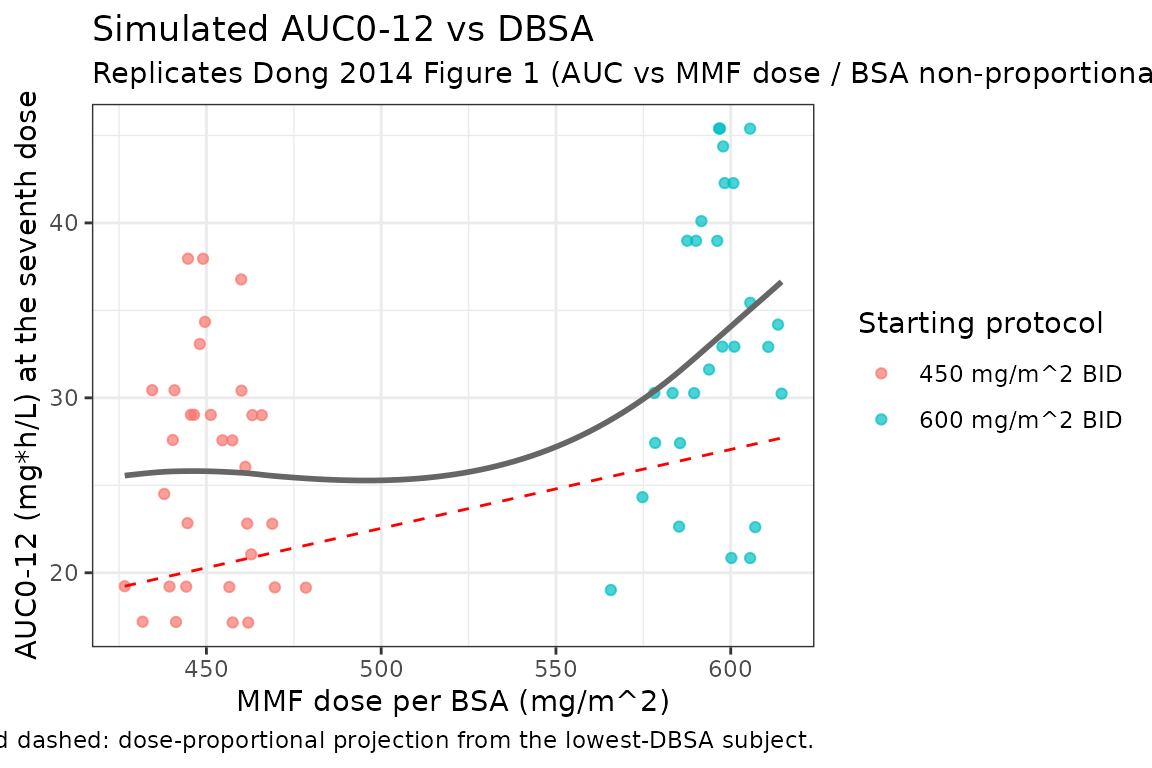
The grey simulated curve lies below the red dose-proportional projection across the DBSA range, reproducing the non-proportionality the paper attributes to the (DBSA/450)^(-0.43) bioavailability factor.
Replicate Figure 3 typical-value profile: MPA concentration vs time
# Pick three subjects spanning the weight range and plot their seventh-dose
# steady-state concentration-time profile to mimic the spread visible in
# the paper's pcVPC.
example_ids <- cohort %>%
  dplyr::arrange(WT) %>%
  dplyr::slice(c(10L, n_subj / 2L, n_subj - 5L)) %>%
  dplyr::pull(id)

sim_ss %>%
  dplyr::filter(id %in% example_ids) %>%
  ggplot(aes(x = time_in_tau, y = Cc, group = id, colour = factor(round(WT, 0)))) +
  geom_line() +
  labs(
    x = "Time after dose (h)",
    y = "MPA plasma concentration (mg/L)",
    title = "Simulated steady-state MPA concentration-time profiles",
    subtitle = "Typical-value model; three example subjects spanning the weight range.",
    colour = "Weight (kg)",
    caption = "Equivalent to one panel of Dong 2014 Figure 3 (pcVPC of population PK)."
  ) +
  theme_bw()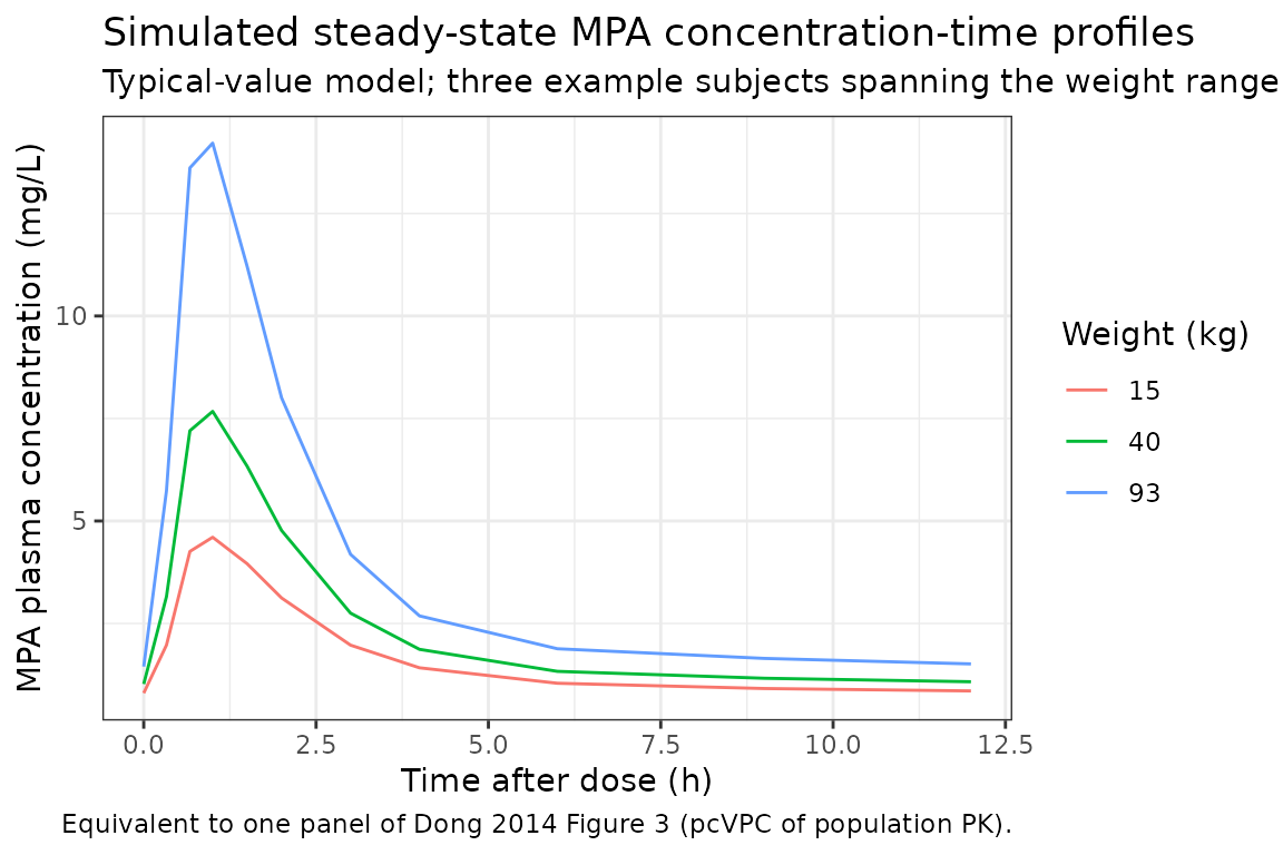
Replicate Figure 5: IMPDH activity vs time
The PD layer’s IMPDH activity curve drops from the baseline E0 (3.45 nmol/h/mg protein) toward 0 during the absorption peak and recovers as MPA washes out. The shape of the curve depends on EC50 = 1.73 mg/L: subjects whose Cmax exceeds EC50 see deep inhibition; subjects with Cmax below EC50 see modest inhibition.
sim_ss %>%
  dplyr::filter(id %in% example_ids) %>%
  ggplot(aes(x = time_in_tau, y = impdh, group = id, colour = factor(round(WT, 0)))) +
  geom_line() +
  geom_hline(yintercept = 3.45, linetype = "dashed", colour = "grey50") +
  labs(
    x = "Time after dose (h)",
    y = "IMPDH activity (nmol/h/mg protein)",
    title = "Simulated IMPDH activity vs time at steady state",
    subtitle = "Inhibitory Emax PD; grey dashed line = E0 = 3.45 nmol/h/mg protein.",
    colour = "Weight (kg)",
    caption = "Equivalent to one panel of Dong 2014 Figure 5 (pcVPC of PK-PD)."
  ) +
  theme_bw()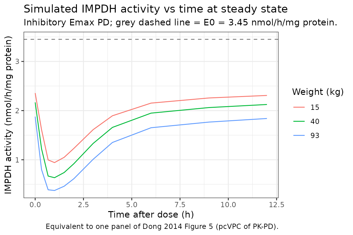
PKNCA validation
PKNCA computes Cmax, Tmax, and AUC0-tau at the seventh (steady-state) dose. The treatment-grouping variable is the starting MMF protocol (450 vs 600 mg/m^2 BID) so per-protocol values can be inspected; both protocols share the same structural PK and differ only in DBSA.
sim_nca <- sim_ss %>%
  dplyr::filter(!is.na(Cc)) %>%
  dplyr::transmute(id, protocol, time = time_in_tau, Cc)

# Defensive time-zero row guarantee per the pknca-recipes.md guidance: the
# extravascular pre-dose concentration is 0. The dense observation grid
# already includes time = 0 in the steady-state window, but the defensive
# bind_rows / distinct pattern protects against future grid changes.
sim_nca <- dplyr::bind_rows(
  sim_nca,
  sim_nca %>% dplyr::distinct(id, protocol) %>%
    dplyr::mutate(time = 0, Cc = 0)
) %>%
  dplyr::distinct(id, protocol, time, .keep_all = TRUE) %>%
  dplyr::arrange(id, protocol, time)

dose_nca <- events %>%
  dplyr::filter(evid == 1L, time == ss_start) %>%
  dplyr::transmute(id, protocol, time = 0, amt)

conc_obj <- PKNCA::PKNCAconc(
  data    = sim_nca,
  formula = Cc ~ time | protocol + id,
  concu   = "mg/L",
  timeu   = "h"
)

dose_obj <- PKNCA::PKNCAdose(
  data    = dose_nca,
  formula = amt ~ time | protocol + id,
  doseu   = "mg"
)

intervals <- data.frame(
  start    = 0,
  end      = tau,
  cmax     = TRUE,
  tmax     = TRUE,
  auclast  = TRUE,
  cav      = TRUE
)

nca_res <- PKNCA::pk.nca(
  PKNCA::PKNCAdata(conc_obj, dose_obj, intervals = intervals)
)

nca_summary_per_protocol <- as.data.frame(nca_res$result) %>%
  dplyr::filter(PPTESTCD %in% c("cmax", "tmax", "auclast", "cav")) %>%
  dplyr::group_by(protocol, PPTESTCD) %>%
  dplyr::summarise(
    median  = stats::median(PPORRES, na.rm = TRUE),
    p05     = stats::quantile(PPORRES, 0.05, na.rm = TRUE),
    p95     = stats::quantile(PPORRES, 0.95, na.rm = TRUE),
    .groups = "drop"
  ) %>%
  dplyr::mutate(
    parameter = dplyr::recode(PPTESTCD,
                              "cmax"    = "Cmax (mg/L)",
                              "tmax"    = "Tmax (h)",
                              "auclast" = "AUC0-tau (mg*h/L)",
                              "cav"     = "Cavg (mg/L)")
  ) %>%
  dplyr::select(protocol, parameter, median, p05, p95)

knitr::kable(
  nca_summary_per_protocol,
  digits  = c(NA, NA, 3, 3, 3),
  caption = "Simulated steady-state NCA per starting MMF protocol (median, 5th and 95th percentiles across the virtual cohort)."
)| protocol | parameter | median | p05 | p95 |
|---|---|---|---|---|
| 450 mg/m^2 BID | AUC0-tau (mg*h/L) | 26.635 | 17.096 | 36.977 |
| 450 mg/m^2 BID | Cavg (mg/L) | 2.220 | 1.425 | 3.081 |
| 450 mg/m^2 BID | Cmax (mg/L) | 7.370 | 3.966 | 11.859 |
| 450 mg/m^2 BID | Tmax (h) | 1.000 | 1.000 | 1.000 |
| 600 mg/m^2 BID | AUC0-tau (mg*h/L) | 32.693 | 20.745 | 44.983 |
| 600 mg/m^2 BID | Cavg (mg/L) | 2.724 | 1.729 | 3.749 |
| 600 mg/m^2 BID | Cmax (mg/L) | 9.230 | 4.856 | 14.676 |
| 600 mg/m^2 BID | Tmax (h) | 1.000 | 1.000 | 1.000 |
The paper does not tabulate explicit Cmax / Tmax / AUC values for direct comparison; AUC was reported per-subject and used to drive the non-proportionality finding in Figure 1 (replicated above), but the source text and tables do not list a pooled-cohort NCA summary that this vignette could match line-by-line. The NCA summary above is therefore a sanity check on the simulated profiles rather than a published-vs-simulated comparison.
Cohort-mean PK-PD summary
A useful end-to-end sanity check is whether the cohort-mean IMPDH
inhibition at the simulated Cmax is consistent with the EC50. With EC50
= 1.73 mg/L and a typical Cmax around 8-12 mg/L (above), the expected
trough IMPDH activity is E0 * EC50 / (EC50 + Cmax), i.e.,
~13-18% of baseline at peak.
cmax_per_subject <- as.data.frame(nca_res$result) %>%
  dplyr::filter(PPTESTCD == "cmax") %>%
  dplyr::transmute(id, protocol, cmax_mg_L = PPORRES)

impdh_at_cmax <- sim_ss %>%
  dplyr::group_by(id) %>%
  dplyr::slice_min(impdh, n = 1, with_ties = FALSE) %>%
  dplyr::ungroup() %>%
  dplyr::select(id, impdh_at_min = impdh)

cmax_per_subject %>%
  dplyr::left_join(impdh_at_cmax, by = "id") %>%
  dplyr::mutate(
    expected_trough  = 3.45 * 1.73 / (1.73 + cmax_mg_L),
    pct_of_baseline  = 100 * impdh_at_min / 3.45
  ) %>%
  dplyr::group_by(protocol) %>%
  dplyr::summarise(
    median_cmax_mg_L      = round(stats::median(cmax_mg_L), 2),
    median_impdh_min      = round(stats::median(impdh_at_min), 3),
    median_pct_baseline   = round(stats::median(pct_of_baseline), 1),
    median_expected_trough= round(stats::median(expected_trough), 3),
    .groups = "drop"
  ) %>%
  knitr::kable(
    caption = "Simulated cohort-median Cmax and the corresponding nadir IMPDH activity (typical-value cohort). The expected trough = E0 * EC50 / (EC50 + Cmax) closely matches the simulated nadir, confirming the inhibitory Emax algebra."
)| protocol | median_cmax_mg_L | median_impdh_min | median_pct_baseline | median_expected_trough |
|---|---|---|---|---|
| 450 mg/m^2 BID | 7.37 | 0.657 | 19.0 | 0.657 |
| 600 mg/m^2 BID | 9.23 | 0.545 | 15.8 | 0.545 |
Assumptions and deviations
-
BSA formula choice. Dong 2014 does not state which
BSA formula was used to compute the per-subject BSA recorded in Table 1;
downstream simulations in this vignette use the Mosteller formula
BSA = sqrt(WT_kg * HT_cm / 3600)with a smooth weight-to-height approximation anchored on paediatric percentiles (10 kg ~ 75 cm, 40 kg ~ 140 cm, 70 kg ~ 168 cm). Users who have actual per-subject BSA values should pass them in directly rather than re-deriving from weight. - Mean transit time vs first-order absorption rate. The model carries both an estimated transit-chain MTT (0.25 h) and a separate first-order absorption rate constant Ka (2.5 /h) from depot to central. This matches the Dong 2014 Methods description (the transit chain feeds the depot, which then empties at Ka into central; the architecture is the same as the Savic 2007 / Wilkins 2008 transit model with first-order absorption in Tikiso 2021 and Smythe 2013).
-
Typical-value figures. The paper reports IIV on Ka
and MTT in excess of 100% CV (299.6% and 144.8% respectively). A fully
stochastic VPC at these levels produces extreme individual profiles; the
typical-value figures above (
zeroRe()) replicate the paper’s median curves cleanly but understate the spread visible in the pcVPC. -
Emax fixed at 0. The paper’s inhibitory Emax model
has Emax (the asymptotic minimum activity) fixed at 0, i.e., complete
IMPDH inhibition is mathematically achievable in the limit of high MPA
concentration. The model file therefore writes the PD equation directly
as
impdh = E0 * EC50 / (EC50 + Cc), which is algebraically equivalent to the paper’s E0 * (1 - Cc / (EC50 + Cc)) form with Emax = 0. -
Covariates screened but not retained. Age, sex,
race, creatinine clearance, serum albumin, hemoglobin, basiliximab
co-medication, and thymoglobulin co-medication were screened in the
source paper’s stepwise selection but did not improve the model and are
not retained in the final structural form; they are recorded in the
model file’s
covariatesDataExcludedfor traceability. Race was borderline-significant on PD baseline E0 (delta-OFV = -8.84) but its bootstrap 95% CI included zero, reflecting the small African-American subset (n = 2 in the PK-PD cohort). - No published NCA summary for line-by-line comparison. The paper reports AUC per-subject (Figure 1 axis) but does not tabulate a cohort Cmax / Tmax / AUC summary. The vignette’s PKNCA table is therefore a simulation sanity check, not a head-to-head paper-vs-simulation comparison.
- Enterohepatic recirculation is not in the structural model. Dong 2014 Discussion explicitly notes the omission: “Firstly, we did not include enterohepatic recirculation in the final model despite the fact that a significant amount can be reabsorbed through this mechanism.” The reported Vp/F estimate (411 L) is higher than other paediatric MPA studies and the paper attributes this in part to the unmodeled enterohepatic recycling.