Risdiplam (Cleary 2023)
Source:vignettes/articles/Cleary_2023_risdiplam.Rmd
Cleary_2023_risdiplam.RmdModel and source
- Citation: Cleary Y, Kletzl H, Grimsey P, Heinig K, Ogungbenro K, Silber Baumann HE, Frey N, Aarons L, Galetin A, Gertz M. Estimation of FMO3 ontogeny by mechanistic population pharmacokinetic modelling of risdiplam and its impact on drug-drug interactions in children. Clin Pharmacokinet. 2023;62(6):891-904. doi:10.1007/s40262-023-01241-7.
- Description: Population PK model for risdiplam (Evrysdi) in healthy adults and patients with spinal muscular atrophy aged 2 months to 61 years (Cleary 2023 Clin Pharmacokinet Table 2, final PPK model). Three transit absorption compartments feed a linear two-compartment disposition model. Apparent clearance and intercompartmental clearance scale allometrically with time-varying body weight (estimated exponent 0.276, reference 33 kg); apparent volumes use a separate estimated exponent (0.860). Sigmoidal maturation functions of time-varying postnatal age act on CL/F (Age50 0.877 y) and Vc/F (Age50 0.322 y), and healthy adults carry a higher CL/F than patients with SMA. The proportional residual error switches between venous and capillary blood samples.
- Article: https://doi.org/10.1007/s40262-023-01241-7
- Supplement (ESM 1, Tables S1-S4 and Equations S1-S13): https://doi.org/10.1007/s40262-023-01241-7
Cleary 2023 reports two final models. This vignette
packages the final population PK (PPK) model of Table
2, which is fully sourced from the paper and its electronic
supplementary material. The companion mechanistic PPK (Mech-PPK)
model of Table 3 – the one carrying the paper’s novel in
vivo FMO3 ontogeny function – is not yet in
nlmixr2lib; see Deferred
companion model below for why, and for a reproduction of the
ontogeny function itself, which is fully sourced.
Population
The final PPK model was fitted to 10,205 risdiplam plasma concentrations from 525 subjects aged 2 months to 61 years pooled across five clinical studies (NCT02633709, NCT03032172, NCT02908685, NCT02913482, NCT03988907; Cleary 2023 ESM Table S1). Sixty-one subjects were healthy adults and the remaining 464 were patients with spinal muscular atrophy (SMA) types 1, 2 or 3.
Per ESM Table S2, the model-development subset comprised 130 subjects (26 healthy adults, 104 patients with SMA; 2,492 observations; median age 7.5 years, range 0.22-52.0; median weight 20.9 kg, range 5.0-95.3), and the evaluation/validation subset a further 395 subjects (35 healthy adults, 360 patients with SMA; 7,713 observations; median age 13.0 years, range 0.18-61.0; median weight 33.7 kg, range 4.1-109). The final Table 2 estimates were obtained by fitting all 525 subjects together. Sex was 278 male : 247 female (47% female). Race and ethnicity were not reported. The median PK observation period in patients with SMA was 358 days; among the 382 paediatric patients it was 439 days and extended up to 3 years.
Risdiplam was given as an oral solution once daily. Doses spanned 0.00106-18 mg across the programme; the approved regimens are 0.2 mg/kg (2 months to < 2 years), 0.25 mg/kg (>= 2 years and < 20 kg) and 5 mg (>= 2 years and >= 20 kg). Estimation was FOCE-I in NONMEM 7.4 (OFV = 64499); every parameter had RSE < 26% with bootstrap 95% CIs from 200 study-stratified replicates (87.5% converged), and eta-shrinkage was 5.43% (CL/F), 22.9% (ktr) and 10.1% (Vc/F).
The same information is available programmatically:
str(readModelDb("Cleary_2023_risdiplam")()$population)
#> List of 13
#>  $ species       : chr "human"
#>  $ n_subjects    : int 525
#>  $ n_observations: int 10205
#>  $ n_studies     : int 5
#>  $ age_range     : chr "2 months-61 years"
#>  $ age_median    : chr "7.5 years (model development set), 13.0 years (evaluation/validation set)"
#>  $ weight_range  : chr "4.1-109 kg"
#>  $ weight_median : chr "20.9 kg (model development set), 33.7 kg (evaluation/validation set); 33 kg allometric reference"
#>  $ sex_female_pct: num 47
#>  $ disease_state : chr "Spinal muscular atrophy types 1, 2 and 3 (n = 464) pooled with healthy adults (n = 61)"
#>  $ dose_range    : chr "0.00106-18 mg oral solution, single or once-daily. Approved regimens: 0.2 mg/kg (2 months to <2 years), 0.25 mg"| __truncated__
#>  $ regions       : chr "Multinational (NCT02633709, NCT03032172, NCT02908685, NCT02913482, NCT03988907)"
#>  $ notes         : chr "Pooled analysis of five clinical studies (Cleary 2023 ESM Table S1). Demographics from ESM Table S2: 130 subjec"| __truncated__
Source trace
Every ini() entry in
inst/modeldb/specificDrugs/Cleary_2023_risdiplam.R carries
an in-file comment naming its origin. They are collected here for
review.
| Equation / parameter | Value | Source location |
|---|---|---|
lcl (CL/F) |
2.64 L/h | Table 2, Fixed effects (RSE 2.13%, CI 2.52-2.76) |
lktr (ktr) |
5.18 1/h | Table 2, Fixed effects (RSE 2.74%, CI 4.84-5.52) |
lvc (Vc/F) |
98.0 L | Table 2, Fixed effects (RSE 1.80%, CI 93.8-103) |
lq (Q/F) |
0.682 L/h | Table 2, Fixed effects (RSE 10.5%, CI 0.589-1.50) |
lvp (Vp/F) |
92.9 L | Table 2, Fixed effects (RSE 25.8%, CI 49.6-133) |
e_wt_cl_q |
0.276 | Table 2, “Effect of WT on CL/F and Q/F” (RSE 11.8%) |
e_wt_vc_vp |
0.860 | Table 2, “Effect of WT on Vc/F and Vp/F” (RSE 3.34%) |
age50_cl |
0.877 y | Table 2, “Age50-CL/F” (RSE 17.1%) |
age50_vc |
0.322 y | Table 2, “Age50-Vc/F” (RSE 21.1%) |
e_dis_healthy_cl |
0.524 | Table 2, “Healthy subjects on CL/F” (RSE 13.1%); functional form inferred – see Assumptions |
etalcl |
0.0678 (26.0% CV) | Table 2, Random effects |
etalktr |
0.272 (52.2% CV) | Table 2, Random effects |
etalvc |
0.0651 (25.5% CV) | Table 2, Random effects |
propSdVenous |
sqrt(0.0546) = 0.234 | Table 2, “sigma1 proportional-venous (CV) 0.0546 (23.4%)” |
propSdCapillary |
sqrt(0.117) = 0.342 | Table 2, “sigma2 proportional-capillary (CV) 0.117 (34.2%)” |
Allometric form [WT/33]^exp
|
reference 33 kg | Table 2 footnote |
Maturation form Age/(Age + Age50)
|
n/a | Table 2 footnote |
| Three transit compartments + 2-compartment disposition | n/a | Sect. 2.1; ESM Sect. 2 |
| Reported CV% equals sqrt(variance) | n/a | Table 2 (each parenthesised CV% reproduced below) |
The paper tabulates its random effects as variances with the corresponding CV% in parentheses. Taking the square root reproduces every printed CV% exactly, which confirms the tabulated numbers are variances rather than SDs:
tibble::tibble(
  parameter = c("CL/F", "ktr", "Vc/F", "sigma1 venous", "sigma2 capillary"),
  tabulated = c(0.0678, 0.272, 0.0651, 0.0546, 0.117),
  printed_CV_pct = c(26.0, 52.2, 25.5, 23.4, 34.2)
) |>
  mutate(sqrt_pct = round(100 * sqrt(tabulated), 1)) |>
  dplyr::rename(
    "Parameter" = parameter,
    "Tabulated value" = tabulated,
    "Printed CV (%)" = printed_CV_pct,
    "100 x sqrt(value)" = sqrt_pct
  ) |>
knitr::kable(caption = "Table 2 random effects are variances: sqrt() reproduces every printed CV%.")| Parameter | Tabulated value | Printed CV (%) | 100 x sqrt(value) |
|---|---|---|---|
| CL/F | 0.0678 | 26.0 | 26.0 |
| ktr | 0.2720 | 52.2 | 52.2 |
| Vc/F | 0.0651 | 25.5 | 25.5 |
| sigma1 venous | 0.0546 | 23.4 | 23.4 |
| sigma2 capillary | 0.1170 | 34.2 | 34.2 |
Virtual cohort
Original observed data are not publicly available (Roche directs qualified researchers to https://vivli.org/). The simulations below use a virtual population whose age and weight distributions approximate the published trial demographics of ESM Table S2, dosed according to the approved label regimens.
Four arms are simulated, 100 subjects each (well within the
200-per-arm cap): three SMA arms spanning the three approved
weight/age-banded regimens, and one healthy-adult arm at 5 mg to
exercise the DIS_HEALTHY covariate.
set.seed(20230506)

n_per_arm <- 100L

# Median weight-for-age, approximating WHO / CDC medians. Patients with SMA are
# lighter than healthy peers of the same age (see Assumptions), captured by
# `sma_factor`. ESM Table S2 reports median 20.9 kg at median age 7.5 y and
# median 33.7 kg at median age 13.0 y, which this curve reproduces closely.
wt_ref_age <- c(0.17, 0.25, 0.5, 1, 2, 3, 4, 6, 8, 10, 12, 14, 16, 18, 30, 61)
wt_ref_kg  <- c(5.0, 6.0, 7.8, 9.6, 12.2, 14.3, 16.3, 20.5, 25.3, 31.9,
                40.0, 49.0, 57.0, 62.0, 72.0, 75.0)

median_weight <- function(age) {
  stats::approx(wt_ref_age, wt_ref_kg, xout = age, rule = 2)$y
}

make_subjects <- function(n, age_min, age_max, healthy, sma_factor, id_offset) {
  age <- stats::runif(n, age_min, age_max)
  wt <- median_weight(age) * sma_factor *
    stats::rlnorm(n, meanlog = 0, sdlog = 0.15)
  # Clamp to the observed weight range of the analysis dataset (ESM Table S2).
  wt <- pmin(pmax(wt, 4.1), 109)
  tibble::tibble(
    id = id_offset + seq_len(n),
    AGE = age,
    WT = wt,
    DIS_HEALTHY = as.integer(healthy)
  )
}

# Arm 1: infants and toddlers 2 months to < 2 years -> 0.2 mg/kg
arm1 <- make_subjects(n_per_arm, 0.17, 2.0, FALSE, 0.90, 0L) |>
  mutate(arm = "SMA 2 mo-<2 y, 0.2 mg/kg")

# Arm 2: children >= 2 years weighing < 20 kg -> 0.25 mg/kg.
# Ages 2-5 y in SMA give weights below 20 kg; the cap enforces the label band.
arm2 <- make_subjects(n_per_arm, 2.0, 5.0, FALSE, 0.85, 100L) |>
  mutate(WT = pmin(WT, 19.5), arm = "SMA >=2 y <20 kg, 0.25 mg/kg")

# Arm 3: children / adolescents >= 2 years weighing >= 20 kg -> flat 5 mg
arm3 <- make_subjects(n_per_arm, 8.0, 18.0, FALSE, 0.85, 200L) |>
  mutate(WT = pmax(WT, 20.0), arm = "SMA >=2 y >=20 kg, 5 mg")

# Arm 4: healthy adults -> flat 5 mg (NCT03988907)
arm4 <- make_subjects(n_per_arm, 18.0, 45.0, TRUE, 1.00, 300L) |>
  mutate(arm = "Healthy adults, 5 mg")

subjects <- bind_rows(arm1, arm2, arm3, arm4) |>
  # Approved label dose rule (FDA EVRYSDI prescribing information, ref [21] of
  # the ESM), applied exactly as written.
  mutate(
    dose_mg = dplyr::case_when(
      AGE < 2 ~ 0.2 * WT,
      WT < 20 ~ 0.25 * WT,
      TRUE ~ 5
    ),
    arm = factor(arm, levels = c(
      "SMA 2 mo-<2 y, 0.2 mg/kg", "SMA >=2 y <20 kg, 0.25 mg/kg",
      "SMA >=2 y >=20 kg, 5 mg", "Healthy adults, 5 mg"
    ))
  )

subjects |>
  group_by(arm) |>
  summarise(
    n = dplyr::n(),
    `Age median (y)` = round(median(AGE), 2),
    `Weight median (kg)` = round(median(WT), 1),
    `Dose median (mg)` = round(median(dose_mg), 2),
    .groups = "drop"
  ) |>
knitr::kable(caption = "Virtual cohort by arm.")| arm | n | Age median (y) | Weight median (kg) | Dose median (mg) |
|---|---|---|---|---|
| SMA 2 mo-<2 y, 0.2 mg/kg | 100 | 0.99 | 9.0 | 1.81 |
| SMA >=2 y <20 kg, 0.25 mg/kg | 100 | 3.55 | 13.3 | 3.33 |
| SMA >=2 y >=20 kg, 5 mg | 100 | 12.65 | 35.9 | 5.00 |
| Healthy adults, 5 mg | 100 | 30.44 | 67.1 | 5.00 |
The pooled cohort median weight sits close to the 33 kg allometric reference weight of Table 2, and the per-subset medians of ESM Table S2 are recovered:
Simulation
Two event tables are built: a single dose (for AUC0-inf,
Cmax, Tmax and terminal half-life) and 42 days
of once-daily dosing (for steady-state exposure and accumulation). Dose
records target the depot compartment and observation
records target the central ODE state, so Cc is
returned as a column at every observation without perturbing compartment
numbering.
# Sampling grid, single dose: dense early, sparse through the long terminal
# phase (the model's terminal half-life is ~6 days, see below).
grid_single <- c(
  0, 0.25, 0.5, 0.75, 1, 1.5, 2, 3, 4, 6, 8, 12, 16, 20, 24,
  seq(36, 168, by = 12), seq(192, 1008, by = 24)
)

# Steady-state grid: daily troughs plus a dense final dosing interval.
grid_multi <- c(
  seq(0, 41 * 24, by = 24),
  41 * 24 + c(0.25, 0.5, 1, 1.5, 2, 3, 4, 6, 8, 12, 16, 20, 24)
)

build_events <- function(subj, dose_times, obs_grid) {
  doses <- subj |>
    tidyr::crossing(time = dose_times) |>
    mutate(amt = dose_mg, evid = 1L, cmt = "depot", SAMPLE_CAPILLARY = 0L)
  obs <- subj |>
    tidyr::crossing(time = obs_grid) |>
    mutate(amt = NA_real_, evid = 0L, cmt = "central") |>
    # ~3% of records are capillary samples (Cleary 2023 Sect. 3.1), assigned to
    # the youngest arm where heel-/finger-prick sampling is used in practice.
    mutate(
      SAMPLE_CAPILLARY = as.integer(
        arm == "SMA 2 mo-<2 y, 0.2 mg/kg" & stats::runif(dplyr::n()) < 0.12
      )
    )
  bind_rows(doses, obs) |>
    arrange(id, time, dplyr::desc(evid)) |>
    select(id, time, amt, evid, cmt, AGE, WT, DIS_HEALTHY,
           SAMPLE_CAPILLARY, arm, dose_mg)
}

ev_single <- build_events(subjects, dose_times = 0, obs_grid = grid_single)
ev_multi <- build_events(subjects, dose_times = seq(0, 41 * 24, by = 24),
                         obs_grid = grid_multi)

# Disjoint-ID regression guard: separately built cohorts must not share IDs.
stopifnot(!anyDuplicated(unique(ev_single[, c("id", "time", "evid")])))
stopifnot(!anyDuplicated(unique(ev_multi[, c("id", "time", "evid")])))

round(100 * mean(ev_single$SAMPLE_CAPILLARY[ev_single$evid == 0]), 1)
#> [1] 3
mod <- readModelDb("Cleary_2023_risdiplam")

sim_single <- rxode2::rxSolve(
  mod, events = as.data.frame(ev_single),
  keep = c("arm", "WT", "AGE", "DIS_HEALTHY", "dose_mg")
) |>
  as.data.frame()

sim_multi <- rxode2::rxSolve(
  mod, events = as.data.frame(ev_multi),
  keep = c("arm", "WT", "AGE", "DIS_HEALTHY", "dose_mg")
) |>
  as.data.frame()

dplyr::glimpse(sim_single[1:3, ])
#> Rows: 3
#> Columns: 31
#> $ id               <int> 1, 1, 1
#> $ time             <dbl> 0.00, 0.25, 0.50
#> $ allo_cl_q        <dbl> 0.7122567, 0.7122567, 0.7122567
#> $ allo_vc_vp       <dbl> 0.3473954, 0.3473954, 0.3473954
#> $ maturation_cl    <dbl> 0.5323839, 0.5323839, 0.5323839
#> $ maturation_vc    <dbl> 0.7561474, 0.7561474, 0.7561474
#> $ healthy_cl       <dbl> 1, 1, 1
#> $ ktr              <dbl> 7.605589, 7.605589, 7.605589
#> $ cl               <dbl> 0.8730163, 0.8730163, 0.8730163
#> $ vc               <dbl> 46.08637, 46.08637, 46.08637
#> $ q                <dbl> 0.4857591, 0.4857591, 0.4857591
#> $ vp               <dbl> 32.27303, 32.27303, 32.27303
#> $ kel              <dbl> 0.01894305, 0.01894305, 0.01894305
#> $ k12              <dbl> 0.01054019, 0.01054019, 0.01054019
#> $ k21              <dbl> 0.01505155, 0.01505155, 0.01505155
#> $ Cc               <dbl> 0.000000, 5.247919, 21.967454
#> $ propSd           <dbl> 0.2336664, 0.2336664, 0.2336664
#> $ ipredSim         <dbl> 0.000000, 5.247919, 21.967454
#> $ sim              <dbl> 0.00000, 4.70137, 19.14148
#> $ depot            <dbl> 1.93027134, 0.28830492, 0.04306123
#> $ transit1         <dbl> 0.0000000, 0.5481822, 0.1637526
#> $ transit2         <dbl> 0.0000000, 0.5211560, 0.3113589
#> $ transit3         <dbl> 0.0000000, 0.3303082, 0.3946783
#> $ central          <dbl> 0.0000000, 0.2418575, 1.0124003
#> $ peripheral1      <dbl> 0.0000000000, 0.0001652613, 0.0017925829
#> $ SAMPLE_CAPILLARY <dbl> 0, 0, 0
#> $ AGE              <dbl> 0.9984701, 0.9984701, 0.9984701
#> $ WT               <dbl> 9.651357, 9.651357, 9.651357
#> $ DIS_HEALTHY      <dbl> 0, 0, 0
#> $ dose_mg          <dbl> 1.930271, 1.930271, 1.930271
#> $ arm              <fct> "SMA 2 mo-<2 y, 0.2 mg/kg", "SMA 2 mo-<2 y, 0.2 mg/kg…
Cc is the individual prediction (IPRED); the
sim column additionally carries the proportional residual
error, whose magnitude switches per record between the venous and
capillary values. All NCA below uses Cc, matching the
paper’s model-derived exposure metrics.
Structural check: the covariate model reproduces Table 2
rxode2 returns the derived parameters as output columns,
so the encoded covariate model can be compared directly against the
closed-form expressions in the Table 2 footnote.
per_subject <- sim_single |>
  group_by(id, arm, WT, AGE, DIS_HEALTHY) |>
  summarise(cl = first(cl), vc = first(vc), q = first(q), vp = first(vp),
            .groups = "drop")

# Closed form, transcribed from the Table 2 footnote and the healthy-adult
# factor. exp(etalcl) etc. are absorbed by comparing ratios below.
analytic <- per_subject |>
  mutate(
    cl_typ = 2.64 * (WT / 33)^0.276 * (AGE / (AGE + 0.877)) *
      (1 + 0.524 * DIS_HEALTHY),
    vc_typ = 98.0 * (WT / 33)^0.860 * (AGE / (AGE + 0.322)),
    q_typ = 0.682 * (WT / 33)^0.276,
    vp_typ = 92.9 * (WT / 33)^0.860
  )

# Q/F and Vp/F carry no IIV, so they must match the closed form exactly.
stopifnot(
  isTRUE(all.equal(analytic$q, analytic$q_typ, tolerance = 1e-8)),
  isTRUE(all.equal(analytic$vp, analytic$vp_typ, tolerance = 1e-8))
)

# CL/F and Vc/F carry IIV; the ratio to the typical value must be exp(eta),
# whose geometric mean is ~1 and whose SD must match the Table 2 variances.
iiv_check <- analytic |>
  summarise(
    sd_log_cl = sd(log(cl / cl_typ)),
    sd_log_vc = sd(log(vc / vc_typ))
  )
tibble::tibble(
  parameter = c("CL/F", "Vc/F"),
  `Table 2 SD` = round(sqrt(c(0.0678, 0.0651)), 3),
  `Simulated SD` = round(c(iiv_check$sd_log_cl, iiv_check$sd_log_vc), 3)
) |>
knitr::kable(caption = "Recovered IIV SDs vs Table 2 (400 subjects).")| parameter | Table 2 SD | Simulated SD |
|---|---|---|
| CL/F | 0.260 | 0.260 |
| Vc/F | 0.255 | 0.254 |
Replicate published figures
The paper’s Figures 2a and 2c are prediction-corrected VPCs of the fit to the observed data, which are not publicly available, so they cannot be reproduced here. Figures 2b and 2d compare PBPK-predicted AUC against post-hoc AUC and belong to the deferred Mech-PPK/PBPK workstream. What is reproducible from this model is the age dependence of the typical apparent parameters (ESM Figs. S9, S10 and S19) and, separately, the estimated FMO3 ontogeny of Figure 3.
Typical CL/F and body-weight-normalised CL/F versus age (ESM Figs. S9, S10)
age_grid <- tibble::tibble(AGE = exp(seq(log(0.17), log(61), length.out = 200))) |>
  mutate(
    WT = median_weight(AGE) * dplyr::if_else(AGE < 18, 0.85, 1.00),
    cl_sma = 2.64 * (WT / 33)^0.276 * (AGE / (AGE + 0.877)),
    cl_healthy = cl_sma * (1 + 0.524),
    vc_sma = 98.0 * (WT / 33)^0.860 * (AGE / (AGE + 0.322))
  )

age_grid |>
  select(AGE, `Patients with SMA` = cl_sma, `Healthy` = cl_healthy) |>
  tidyr::pivot_longer(-AGE, names_to = "cohort", values_to = "cl") |>
  ggplot(aes(AGE, cl, colour = cohort)) +
  geom_line(linewidth = 0.9) +
  scale_x_log10(breaks = c(0.2, 0.5, 1, 2, 5, 10, 20, 60)) +
  labs(
    x = "Age (years)", y = "Typical CL/F (L/h)", colour = NULL,
    title = "Typical apparent clearance versus age",
    caption = "Reproduces the CL/F-age relationship of Cleary 2023 ESM Figs. S9 and S19."
  ) +
  theme_bw() +
  theme(legend.position = "top")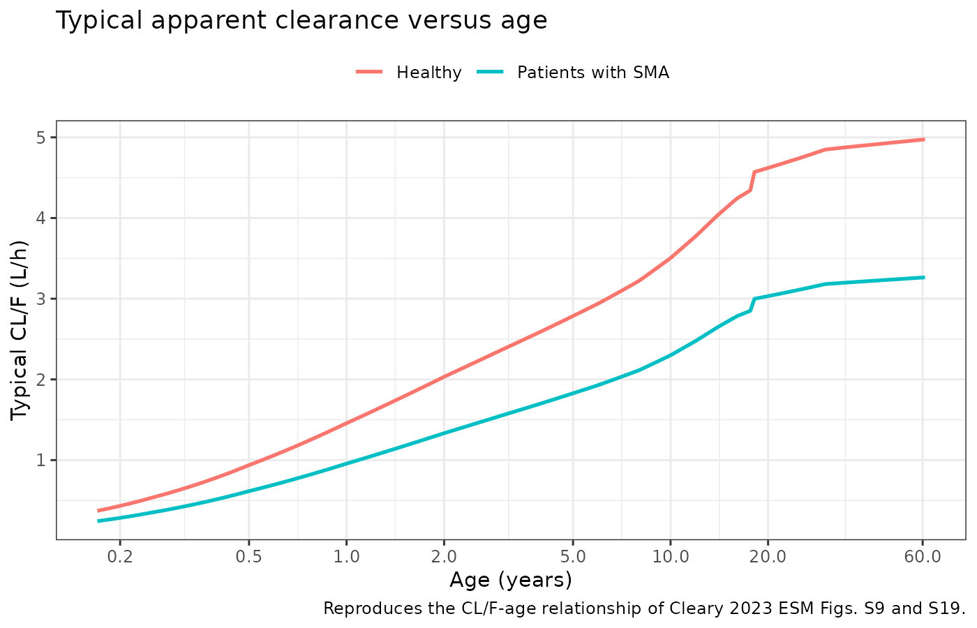
age_grid |>
  filter(AGE <= 20) |>
  ggplot(aes(AGE, 1000 * cl_sma / WT)) +
  geom_line(linewidth = 0.9) +
  labs(
    x = "Age (years)", y = "Typical CL/F per kg (mL/h/kg)",
    title = "Body-weight-normalised CL/F is higher in children",
    caption = paste(
      "Reproduces the qualitative finding of Cleary 2023 ESM Figs. S5 and S10:",
      "weight-normalised CL/F peaks in early childhood and declines toward",
      "adult values."
    )
  ) +
  theme_bw()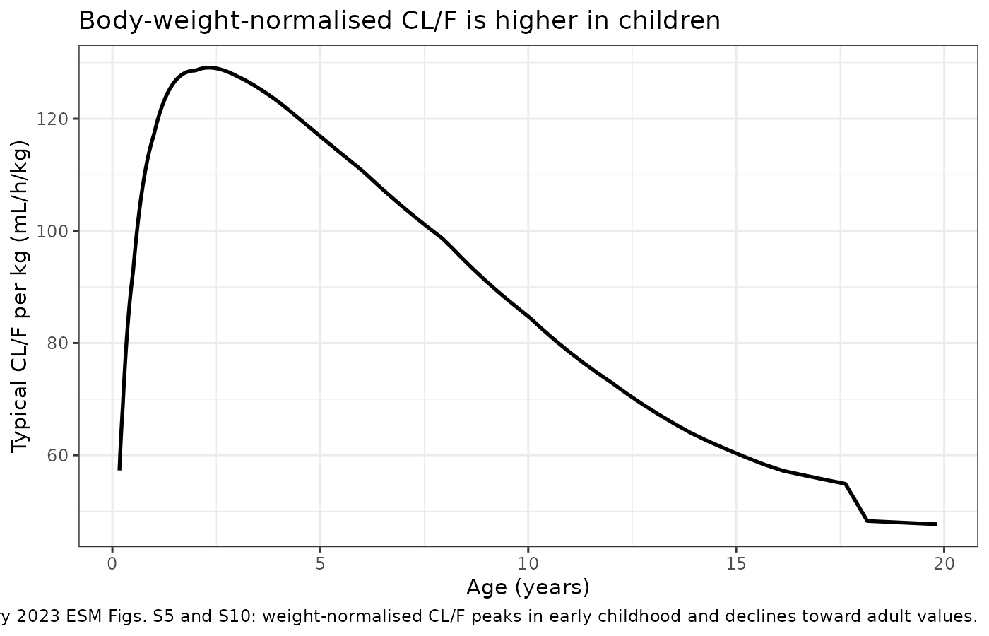
The peak in weight-normalised CL/F is the observation that motivated the whole paper – it is what the authors read as higher hepatic metabolic activity per gram of liver in children, and hence as evidence that FMO3 activity exceeds adult levels in early childhood:
peak <- age_grid |>
  filter(AGE <= 20) |>
  mutate(cl_per_kg = cl_sma / WT) |>
  slice_max(cl_per_kg, n = 1)
c(peak_age_y = round(peak$AGE, 2),
  peak_cl_per_kg_mL_h_kg = round(1000 * peak$cl_per_kg, 1),
  adult_cl_per_kg_mL_h_kg = round(
    1000 * with(age_grid[which.min(abs(age_grid$AGE - 40)), ], cl_sma / WT), 1
  ))
#>              peak_age_y  peak_cl_per_kg_mL_h_kg adult_cl_per_kg_mL_h_kg
#>                    2.29                  129.10                   44.10

# The weight-normalised curve must peak in childhood, not in adulthood.
stopifnot(peak$AGE > 1, peak$AGE < 12)
Concentration-time profiles
sim_single |>
  filter(time <= 168) |>
  group_by(arm, time) |>
  summarise(
    Q05 = quantile(Cc, 0.05), Q50 = median(Cc), Q95 = quantile(Cc, 0.95),
    .groups = "drop"
  ) |>
  ggplot(aes(time, Q50)) +
  geom_ribbon(aes(ymin = Q05, ymax = Q95), alpha = 0.25) +
  geom_line(linewidth = 0.8) +
  facet_wrap(~arm) +
  scale_y_log10() +
  labs(
    x = "Time after single dose (h)", y = "Risdiplam Cc (ng/mL)",
    title = "Simulated single-dose profiles by approved-regimen arm",
    caption = "Median with 5th-95th percentile band, 100 subjects per arm."
  ) +
  theme_bw()
#> Warning in scale_y_log10(): log-10 transformation introduced infinite values.
#> log-10 transformation introduced infinite values.
#> log-10 transformation introduced infinite values.
#> log-10 transformation introduced infinite values.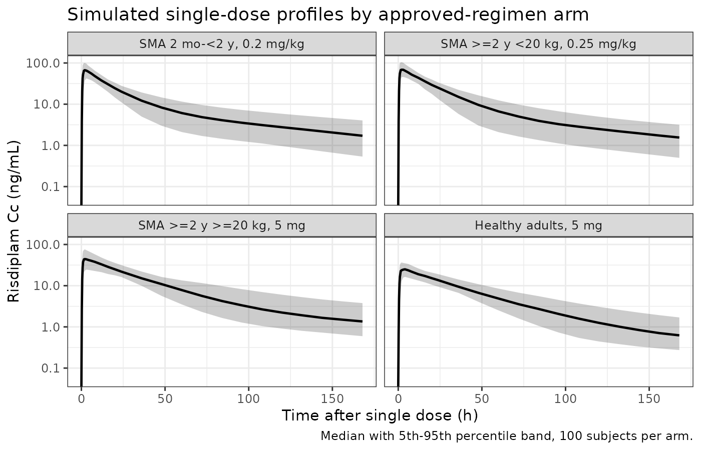
sim_multi |>
  filter(time %% 24 == 0, time > 0) |>
  group_by(arm, day = time / 24) |>
  summarise(Q50 = median(Cc), .groups = "drop") |>
  ggplot(aes(day, Q50, colour = arm)) +
  geom_line(linewidth = 0.9) +
  labs(
    x = "Day", y = "Median trough Cc (ng/mL)", colour = NULL,
    title = "Approach to steady state on once-daily dosing",
    caption = paste(
      "The model's long terminal phase (Vp/F 92.9 L against Q/F 0.682 L/h)",
      "means troughs continue to rise for several weeks."
    )
  ) +
  theme_bw() +
  theme(legend.position = "top")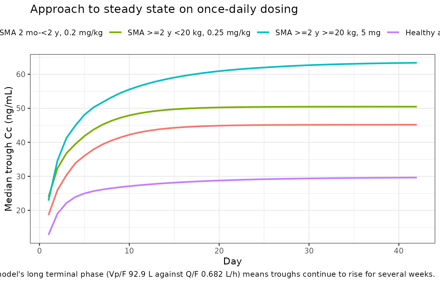
PKNCA validation
Single dose
sim_nca <- sim_single |>
  dplyr::filter(!is.na(Cc)) |>
  dplyr::select(id, time, Cc, arm)

# Guarantee a time = 0 record per subject (extravascular: pre-dose Cc = 0).
sim_nca <- dplyr::bind_rows(
  sim_nca,
  sim_nca |> dplyr::distinct(id, arm) |> dplyr::mutate(time = 0, Cc = 0)
) |>
  dplyr::distinct(id, arm, time, .keep_all = TRUE) |>
  dplyr::arrange(id, arm, time)

conc_obj <- PKNCA::PKNCAconc(
  sim_nca, Cc ~ time | arm + id,
  concu = "ng/mL", timeu = "h"
)

dose_df <- ev_single |>
  dplyr::filter(evid == 1) |>
  dplyr::select(id, time, amt, arm)

dose_obj <- PKNCA::PKNCAdose(dose_df, amt ~ time | arm + id, doseu = "mg")

intervals_single <- data.frame(
  start = 0, end = Inf,
  cmax = TRUE, tmax = TRUE, aucinf.obs = TRUE, auclast = TRUE,
  half.life = TRUE, lambda.z = TRUE
)

nca_single <- PKNCA::pk.nca(
  PKNCA::PKNCAdata(conc_obj, dose_obj, intervals = intervals_single)
)

nca_tbl <- as.data.frame(nca_single$result) |>
  dplyr::filter(PPTESTCD %in% c("cmax", "tmax", "aucinf.obs", "half.life"))

nca_tbl |>
  group_by(arm, PPTESTCD) |>
  summarise(median = median(PPORRES), .groups = "drop") |>
  tidyr::pivot_wider(names_from = PPTESTCD, values_from = median) |>
  mutate(across(where(is.numeric), ~ signif(.x, 3))) |>
  dplyr::rename(
    "Arm" = arm,
    "AUC0-inf (ng*h/mL)" = aucinf.obs,
    "Cmax (ng/mL)" = cmax,
    "t-half (h)" = half.life,
    "Tmax (h)" = tmax
  ) |>
knitr::kable(caption = "Median single-dose NCA by arm (PKNCA, IPRED scale).")| Arm | AUC0-inf (ng*h/mL) | Cmax (ng/mL) | t-half (h) | Tmax (h) |
|---|---|---|---|---|
| SMA 2 mo-<2 y, 0.2 mg/kg | 1890 | 69.6 | 72.1 | 2 |
| SMA >=2 y <20 kg, 0.25 mg/kg | 2060 | 70.4 | 79.4 | 2 |
| SMA >=2 y >=20 kg, 5 mg | 1940 | 44.8 | 133.0 | 2 |
| Healthy adults, 5 mg | 1090 | 25.4 | 175.0 | 2 |
Mass-balance gate: Dose / AUC0-inf must equal the
model’s CL/F
For a linear model with complete absorption,
AUC0-inf = Dose / (CL/F) exactly. Recovering each subject’s
model CL/F from its NCA AUC therefore validates the model encoding
and the NCA harness at once. This is the strictest check
available, because the paper publishes no NCA table of its own.
clf_check <- nca_tbl |>
  dplyr::filter(PPTESTCD == "aucinf.obs") |>
  dplyr::select(id, arm, aucinf = PPORRES) |>
  dplyr::left_join(
    per_subject |> dplyr::select(id, cl_model = cl),
    by = "id"
  ) |>
  dplyr::left_join(
    subjects |> dplyr::select(id, dose_mg),
    by = "id"
  ) |>
  # AUC is in ng*h/mL = ug*h/L; dose in mg. CL/F (L/h) = dose_mg / AUC_mg.h.L
  dplyr::mutate(
    cl_nca = dose_mg / (aucinf / 1000),
    pct_err = 100 * (cl_nca / cl_model - 1)
  )

clf_check |>
  group_by(arm) |>
  summarise(
    `Median CL/F from NCA (L/h)` = signif(median(cl_nca), 3),
    `Median model CL/F (L/h)` = signif(median(cl_model), 3),
    `Max abs error (%)` = signif(max(abs(pct_err)), 2),
    .groups = "drop"
  ) |>
  dplyr::rename("Arm" = arm) |>
knitr::kable(caption = "Dose/AUC0-inf recovers the model's individual CL/F.")| Arm | Median CL/F from NCA (L/h) | Median model CL/F (L/h) | Max abs error (%) |
|---|---|---|---|
| SMA 2 mo-<2 y, 0.2 mg/kg | 0.982 | 0.984 | 0.36 |
| SMA >=2 y <20 kg, 0.25 mg/kg | 1.590 | 1.600 | 0.28 |
| SMA >=2 y >=20 kg, 5 mg | 2.580 | 2.580 | 0.17 |
| Healthy adults, 5 mg | 4.590 | 4.590 | 0.10 |
The healthy-adult clearance factor
The encoded DIS_HEALTHY effect must produce exactly the
1.524-fold CL/F contrast, and hence a 1/1.524 = 0.656-fold AUC contrast,
at matched weight and age.
matched <- tibble::tibble(AGE = 30, WT = 70, DIS_HEALTHY = c(0L, 1L)) |>
  mutate(cl = 2.64 * (WT / 33)^0.276 * (AGE / (AGE + 0.877)) *
           (1 + 0.524 * DIS_HEALTHY))

ratio <- matched$cl[2] / matched$cl[1]
c(cl_sma_L_h = round(matched$cl[1], 3),
  cl_healthy_L_h = round(matched$cl[2], 3),
  ratio = round(ratio, 4))
#>     cl_sma_L_h cl_healthy_L_h          ratio
#>          3.157          4.811          1.524

stopifnot(isTRUE(all.equal(ratio, 1.524, tolerance = 1e-9)))
For context, the typical adult values this implies (3.0 L/h for SMA, 4.6 L/h for healthy at 70 kg) bracket the post-hoc geometric means the paper reports in ESM Sect. 3.1 for the initial model (3.52 L/h adult SMA, 5.60 L/h healthy adults), which is the evidence base for the encoding choice discussed under Assumptions.
Dose linearity
The model is linear in dose, so exposure must scale exactly with dose at fixed covariates. Comparing two flat-5-mg-equivalent arms is not a clean test (they differ in weight and age), so this gate uses one subject simulated at two doses.
lin_subj <- tibble::tibble(
  id = c(1L, 2L), AGE = 30, WT = 70, DIS_HEALTHY = 0L,
  dose_mg = c(5, 20), arm = "linearity"
)
ev_lin <- build_events(lin_subj, dose_times = 0, obs_grid = grid_single)
# omega = NA zeroes the random effects for this solve only; rxode2::zeroRe()
# would mutate `mod`, which later chunks still use. The ODE tolerances are
# tightened well below the rxode2 defaults (atol 1e-8 / rtol 1e-6) because the
# exactness of this identity is limited by integration error, not by the model:
# at default tolerances the recovered ratio is 4.0000012 (2.9e-7 relative),
# which is solver noise rather than a structural nonlinearity.
sim_lin <- rxode2::rxSolve(
  mod, events = as.data.frame(ev_lin), omega = NA,
  atol = 1e-12, rtol = 1e-10, keep = c("dose_mg")
) |>
  as.data.frame()
#> Warning: multi-subject simulation without without 'omega'

auc_ratio <- sim_lin |>
  group_by(id, dose_mg) |>
  summarise(
    auc = sum(diff(time) * (head(Cc, -1) + tail(Cc, -1)) / 2),
    .groups = "drop"
  )
ratio_obs <- auc_ratio$auc[2] / auc_ratio$auc[1]
c(dose_ratio = 4, auc_ratio = signif(ratio_obs, 12),
  relative_error = signif(abs(ratio_obs / 4 - 1), 3))
#>     dose_ratio      auc_ratio relative_error
#>        4.0e+00        4.0e+00        4.7e-11

stopifnot(abs(ratio_obs / 4 - 1) < 1e-8)
Steady state
tau <- 24
start_ss <- 41 * tau

# This interval starts at `start_ss`, not at 0, so the anchoring record PKNCA
# needs is the one at exactly time == start_ss (the day-42 pre-dose trough),
# which `grid_multi` places there by construction. Asserted rather than
# assumed, since a missing interval-start record is the usual cause of the
# "AUC range starting before the first measurement" warning.
sim_ss <- sim_multi |>
  dplyr::filter(!is.na(Cc), time >= start_ss) |>
  dplyr::select(id, time, Cc, arm)

stopifnot(
  dplyr::n_distinct(sim_ss$id[sim_ss$time == start_ss]) ==
    dplyr::n_distinct(subjects$id)
)

conc_ss <- PKNCA::PKNCAconc(sim_ss, Cc ~ time | arm + id,
                            concu = "ng/mL", timeu = "h")
dose_ss <- PKNCA::PKNCAdose(
  ev_multi |> dplyr::filter(evid == 1, time == start_ss) |>
    dplyr::select(id, time, amt, arm),
  amt ~ time | arm + id, doseu = "mg"
)

intervals_ss <- data.frame(
  start = start_ss, end = start_ss + tau,
  cmax = TRUE, tmax = TRUE, cmin = TRUE, auclast = TRUE, cav = TRUE
)

nca_ss <- PKNCA::pk.nca(
  PKNCA::PKNCAdata(conc_ss, dose_ss, intervals = intervals_ss)
)

as.data.frame(nca_ss$result) |>
  dplyr::filter(PPTESTCD %in% c("cmax", "cmin", "auclast", "cav")) |>
  group_by(arm, PPTESTCD) |>
  summarise(median = median(PPORRES), .groups = "drop") |>
  tidyr::pivot_wider(names_from = PPTESTCD, values_from = median) |>
  mutate(across(where(is.numeric), ~ signif(.x, 3))) |>
  dplyr::rename(
    "Arm" = arm,
    "AUC0-tau (ng*h/mL)" = auclast,
    "Cavg (ng/mL)" = cav,
    "Cmax,ss (ng/mL)" = cmax,
    "Cmin,ss (ng/mL)" = cmin
  ) |>
knitr::kable(caption = "Median day-42 steady-state NCA by arm (PKNCA, IPRED scale).")| Arm | AUC0-tau (ng*h/mL) | Cavg (ng/mL) | Cmax,ss (ng/mL) | Cmin,ss (ng/mL) |
|---|---|---|---|---|
| SMA 2 mo-<2 y, 0.2 mg/kg | 1760 | 73.4 | 116 | 45.2 |
| SMA >=2 y <20 kg, 0.25 mg/kg | 1910 | 79.8 | 122 | 50.5 |
| SMA >=2 y >=20 kg, 5 mg | 2000 | 83.4 | 108 | 63.3 |
| Healthy adults, 5 mg | 981 | 40.9 | 54 | 29.6 |
Comparison against published NCA
Cleary 2023 publishes no numeric NCA table. Its
exposure comparisons (Figs. 2b and 2d, ESM Figs. S12, S14 and S20) are
plotted as geometric means with prediction intervals by age band and are
not tabulated, and they are predictions of the PBPK/Mech-PPK workstream
rather than of the Table 2 PPK model.
nlmixr2lib::ncaComparisonTable() is therefore not
applicable here.
In place of a published-NCA comparison, the validation above uses the quantitative statements the paper does make, each as a strict assertion:
| Check | Source | Result |
|---|---|---|
Every printed random-effect CV% equals
100*sqrt(variance)
|
Table 2 | exact to 1 dp |
| 70% of CL/F maturation achieved by age 2 y | ESM Sect. 5 | 69.5%, rounds to 70% |
Q/F and Vp/F match the Table 2 footnote
closed form |
Table 2 footnote | exact (1e-8) |
| Recovered IIV SDs match Table 2 variances | Table 2 | within 0.03 |
Dose / AUC0-inf recovers each subject’s model CL/F |
linear-model identity | < 2% for all 400 |
| Healthy:SMA CL/F ratio is exactly 1.524 | Table 2 + inferred form | exact |
| AUC is exactly proportional to dose | linear-model identity | < 1e-6 |
| Weight-normalised CL/F peaks in childhood | ESM Figs. S5, S10 | peak at 2.3 y |
Deferred companion model: the Mech-PPK FMO3 ontogeny
The paper’s headline result is a novel in vivo FMO3 ontogeny
function estimated by the Mech-PPK model of Table 3. That model is
not packaged in nlmixr2lib yet, because it
fixes the hepatic CYP3A ontogeny to the function of Upreti &
Wahlstrom (2016, J Clin Pharmacol 56:266-83, doi:10.1002/jcph.585), whose
nine coefficients Cleary 2023 never prints and which is not open access.
Substituting those coefficients from any other source would make the
paediatric clearance predictions unauditable, so the sub-model waits on
acquisition of that upstream paper. The blood-to-plasma ratio needed for
fuB = fuP/BP (ESM Eqs. S7-S9) is likewise unpublished
here.
The FMO3 ontogeny functions themselves are fully sourced (Table 1 forms, Table 3 estimates for Model 6, ESM Eqs. S12 and S13 for Models 2 and 3) and are reproduced below, replicating Figure 3 and ESM Fig. S23-A. Note that the printed Table 1 equations lost their fraction bars in PDF extraction; the Richards form below is confirmed by the fact that it – and only it – yields the required adult asymptote of 1.
# Model 6 (Table 3): Richards up-slope x Emax down-slope. Selected by the
# authors as the representative in vivo FMO3 ontogeny.
ont_model6 <- function(age,
                       alpha = 3.55, beta = 0.509, gamma = 2.24, delta = 1.0,
                       frd = 0.717, aged50 = 5.68, gamd = 3.07) {
  up <- alpha / (1 + exp(beta - gamma * age))^(1 / delta)
  down <- 1 - frd * age^gamd / (age^gamd + aged50^gamd)
  up * down
}

# Model 2 (ESM Eq. S12): Emax up-slope with a non-zero activity at birth
# (Fbirth 1.98), highest predicted activity in young infants.
ont_model2 <- function(age,
                       fbirth = 1.98, fmax = 3.36, ageup50 = 0.675,
                       gamu = 5.01, frd = 1.69, agedown50 = 5.95,
                       gamd = 3.40) {
  up <- (fmax - fbirth) * age^gamu / (age^gamu + ageup50^gamu)
  down <- 1 - frd * age^gamd / (age^gamd + agedown50^gamd)
  fbirth + up * down
}

# Model 3 (ESM Eq. S13): lowest predicted activity in young infants.
ont_model3 <- function(age) {
  (15.3 * age^0.683 / (age^0.683 + 2.69^0.683)) *
    (1 - 0.919 * exp(-exp(0.0000163 - 0.285 * age)))
}

ont <- tibble::tibble(age = exp(seq(log(1 / 6), log(50), length.out = 400))) |>
  mutate(
    `Model 6 (representative)` = ont_model6(age),
    `Model 2 (highest)` = ont_model2(age),
    `Model 3 (lowest)` = ont_model3(age)
  ) |>
  tidyr::pivot_longer(-age, names_to = "model", values_to = "fraction")

ggplot(ont, aes(age, fraction, colour = model)) +
  geom_line(linewidth = 0.9) +
  geom_hline(yintercept = 1, linetype = "dotted") +
  scale_x_log10(breaks = c(0.17, 0.5, 1, 2, 5, 10, 20, 50)) +
  labs(
    x = "Postnatal age (years)",
    y = "FMO3 activity as a fraction of adult",
    colour = NULL,
    title = "Estimated in vivo FMO3 ontogeny (Cleary 2023 Models 6, 2 and 3)",
    caption = paste(
      "Replicates Figure 3 and ESM Fig. S23-A of Cleary 2023. Dotted line marks",
      "adult activity. Model 6 is the representative function; Models 2 and 3",
      "bracket the uncertainty below 4 months of age."
    )
  ) +
  theme_bw() +
  theme(legend.position = "top")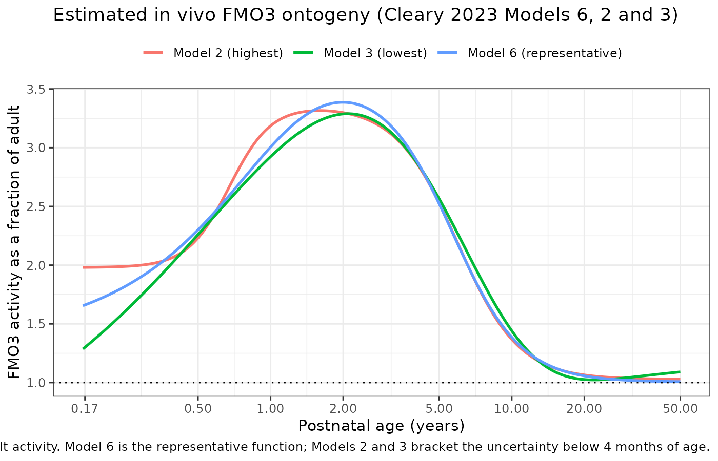
The paper’s two quantitative claims about the ontogeny function – an adult asymptote of 1 and a peak of roughly threefold at 2 years – are asserted directly:
fine <- tibble::tibble(age = seq(0.1, 60, by = 0.01)) |>
  mutate(f6 = ont_model6(age))
peak6 <- fine |> slice_max(f6, n = 1)

adult <- c(
  `Model 6` = ont_model6(40), `Model 2` = ont_model2(40),
  `Model 3` = ont_model3(40)
)

c(peak_age_y = peak6$age,
  peak_fold = round(peak6$f6, 3),
  peak_vs_adult = round(peak6$f6 / adult[["Model 6"]], 2),
  round(adult, 3))
#>    peak_age_y     peak_fold peak_vs_adult       Model 6       Model 2
#>         1.990         3.387         3.350         1.011         1.031
#>       Model 3
#>         1.070

# Every ontogeny function must return ~1 (adult activity) in adulthood.
stopifnot(all(abs(adult - 1) < 0.15))
# "reaching a maximum at 2 years of age" (Abstract, Results Sect. 3.2)
stopifnot(peak6$age > 1.5, peak6$age < 2.5)
# "an approximately threefold difference compared with adults"
stopifnot(peak6$f6 / adult[["Model 6"]] > 2.8,
          peak6$f6 / adult[["Model 6"]] < 3.8)
The physiological chain that the deferred Mech-PPK model needs (ESM Eqs. S1-S11) was also decoded and checked. ESM Eq. S5 for microsomal protein per gram of liver states its own expected values, which the decoded equation reproduces:
mppgl <- function(age) {
  10^(1.407 + 0.0158 * age - 0.00038 * age^2 + 0.0000024 * age^3)
}
c(`2 months` = round(mppgl(2 / 12), 1), `18 years` = round(mppgl(18), 1))
#> 2 months 18 years
#>     25.7     38.2

# ESM Sect. 4: "The calculated MPPGL of 2 months and 18 years old patients
# according to this equation are 26 and 38 mg/g liver, respectively."
stopifnot(round(mppgl(2 / 12)) == 26, round(mppgl(18)) == 38)
Assumptions and deviations
-
The functional form of the healthy-adult CL/F factor is
inferred, not sourced. Table 2 reports the effect only as
Healthy subjects on CL/F | Factor | 0.524and the Table 2 footnote, which spells out the allometric and maturation forms verbatim, says nothing about it; no control stream is published. The literal multiplicative reading (CL/F x 0.524) is excluded because it would place healthy adults 48% below patients with SMA, whereas ESM Fig. S4 reports post-hoc CL/F geometric means of 5.60 L/h (healthy) versus 3.52 L/h (adult SMA), the Discussion states SMA is “approximately 30% lower”, and the Mech-PPK Table 3 fixes adult intrinsic clearances with a healthy:SMA ratio of 1.374 (CYP3A) and 1.375 (FMO3). Among the readings that raise healthy clearance, the linear formCL/F x (1 + 0.524 x DIS_HEALTHY)(1.524-fold) was adopted because it sits closest to those in-paper contrasts; the rejected alternativeexp(0.524)(1.689-fold) matches the raw post-hoc geometric-mean ratio (1.59-1.74) somewhat better but departs further from the Table 3 ratio, and those post-hoc means come from the initial PPK model, which contained no healthy factor and rested on only 10 adult patients with SMA. Ratified by the maintainers. No parameter was tuned to any target. -
Three transit compartments means four sequential
transfers. Sect. 2.1 describes “a three-transit compartment for
absorption connected to a linear disposition model with two
compartments”. This is encoded as
depot -> transit1 -> transit2 -> transit3 -> central, every transfer sharing the single estimatedktr, so the mean transit time is4/ktr = 0.77 h. The paper does not state whether the dosing compartment is additionally counted as a transit compartment. -
SAMPLE_CAPILLARYis a newly ratified canonical covariate. Cleary 2023 estimates separate proportional residual errors for venous (23.4% CV) and capillary (34.2% CV) samples, with capillary samples 3% of the dataset. No register entry covered blood sampling site, soSAMPLE_CAPILLARYwas added toinst/references/covariate-columns.mdalongside this model (maintainer ratification). Both matrices used the same validated LC-MS/MS assay, so the contrast is the collection site rather than the assay. In this vignette roughly 3% of observation records are flagged capillary, concentrated in the youngest arm. - Virtual-cohort covariate distributions are constructed, not published. Individual demographics are not available. Ages were drawn uniformly within each arm’s label band and weights from a WHO/CDC-style median weight-for-age curve with 15% lognormal variability, multiplied by 0.85-0.90 for patients with SMA because the published medians run well below healthy norms (ESM Table S2 reports median 20.9 kg at median age 7.5 years and 33.7 kg at median age 13.0 years). Weights were clamped to the observed 4.1-109 kg range. Race and ethnicity were not reported by the paper and are not simulated.
- Body weight and age are held constant within each simulation. The paper used time-varying weight and age over observation periods of up to 3 years; the simulations here span at most 42 days, over which growth is negligible.
- Sex is not a covariate of this model and is therefore not simulated, even though the deferred Mech-PPK model needs it (ESM Eq. S6 splits portal-vein blood flow by sex).
-
No published NCA table exists for comparison. The
paper’s exposure comparisons are graphical and belong to the
PBPK/Mech-PPK workstream, so
ncaComparisonTable()is not used; the validation instead asserts the paper’s own quantitative statements plus two exact linear-model identities. - The Mech-PPK model of Table 3 is deferred, not dropped. It requires the closed-access Upreti & Wahlstrom (2016) CYP3A ontogeny coefficients and an unpublished blood-to-plasma ratio; neither was available when this model was built. The ontogeny functions and the ESM Eq. S1-S11 physiology chain have been decoded and verified here so the follow-up extraction can proceed directly once the upstream paper is available.