Model and source
- Citation: Ji T, Chen X, Liu X, Yeleswaram S. Population Pharmacokinetics Analysis of Pemigatinib in Patients With Advanced Malignancies. Clin Pharmacol Drug Dev. 2022;11(4):454-466.
- Article: https://doi.org/10.1002/cpdd.1038 (open access, PMC9306536)
Pemigatinib is an oral inhibitor of fibroblast growth factor
receptors 1-3, approved for previously treated cholangiocarcinoma with
an FGFR2 fusion or rearrangement at 13.5 mg once daily, 2 weeks
on and 1 week off. Ji 2022 is the first population PK analysis of
pemigatinib: a two-compartment model with first-order absorption and
linear elimination. A later, larger analysis of the same programme (Gong
2023, seven studies, sequential zero-/first-order absorption) is
packaged separately as Gong_2023_pemigatinib.
mod <- readModelDb("Ji_2022_pemigatinib")Population
The analysis pooled 2968 plasma concentrations from 318 patients in three studies (Ji 2022 Table 1 and Results “Data Description”): FIGHT-101, a phase 1/2 dose-escalation/expansion study in advanced malignancies (157 patients, 1-20 mg once daily, rich sampling); FIGHT-102, a phase 1 study in Japanese patients (25 patients, 9 and 13.5 mg, rich sampling); and FIGHT-202, a phase 2 study in previously treated cholangiocarcinoma (136 patients, 13.5 mg, sparse sampling). Median (range) age was 59 (21-79) years and median (range) body weight 73.3 (39.8-156.0) kg; 55.0% were women; 68.2% were White, 8.8% Japanese, 7.2% other Asian, 6.3% Black and 6.0% Hispanic (Table 2). Renal function was normal in 45.9%, mildly impaired in 42.1% and moderately impaired in 11.9%; hepatic function was normal in 67.0%, mildly impaired in 29.6% and moderately impaired in 3.5%. Co-medications (Table 3) included phosphate binders (36.1%) used to manage on-target hyperphosphatemia, proton-pump inhibitors (PPIs, 26.9%) and H2-receptor antagonists (11.1%).
Source trace
| Model element | Value | Source |
|---|---|---|
| Structure: 2-compartment, first-order absorption, linear elimination | – | Results “Base Structure Model” and “Final Model” |
lka |
log(1.49) 1/h | Table 4; Equation IV |
lcl |
log(9.00) L/h | Table 4; Equation I |
lvc |
log(161) L | Table 4; Equation II |
lvp |
log(80.1) L | Table 4; Equation III |
lq |
log(16.0) L/h | Table 4 |
e_phosbinder_cl |
0.141, as (1 + 0.141 (1 - BINDER))
|
Table 4 “Phosphate binder on CL”; Equation I |
e_sex_cl |
0.190, as (1 + 0.19 (1 - SEXN))
|
Table 4 “Sex (male vs female) on CL”; Equation I |
e_sex_ka |
0.565, as (1 - 0.565 (1 - SEXN))
|
Equation IV (not tabulated in Table 4) |
e_ppi_vc |
-0.244, as (1 - 0.244 (1 - PPI))
|
Table 4 “Proton pump inhibitor on Vc/F”; Equation II |
e_wt_vc |
0.738 on (WT/73.3) | Table 4; Equation II |
e_wt_vp |
1.22 on (WT/73.3) | Table 4; Equation III |
etalcl, etalvc
|
0.434^2, 0.351^2; covariance 0.122 | Table 4 IIV %CV and “Omega matrix for CL/F and Vc/F” |
etalka |
1.27^2 | Table 4 IIV %CV |
expSd |
0.401 (log scale) | Table 4 “RV,SD”; Results “Base Structure Model” (log-transformed data) |
| SEXN coding 1 = male, 2 = female; BINDER 1 = used | – | “Where:” block below Equations I-IV |
| Reference body weight 73.3 kg | – | Equations II-III; Table 2 median |
Reading the IIV %CV as sqrt(omega^2)
Table 4 lists IIV as %CV with a %RSE and a bootstrap 95% CI. The
discriminating row is ka (127 %CV, %RSE 12.3, CI 112-143). If the %RSE
refers to the variance omega^2 = 1.27^2 = 1.613, its
delta-method CI on the sqrt(omega^2) scale is
127 +/- 1.96 * 127 * 0.123 / 2, i.e. 112-142, which
reproduces the printed interval. Under the alternative reading
CV = sqrt(exp(omega^2) - 1) the same %RSE gives 103-151.
The model therefore uses omega^2 = (CV/100)^2. With these
variances the CL/F-Vc/F covariance of 0.122 corresponds to a correlation
of 0.80.
om <- c(cl = 0.434^2, vc = 0.351^2, ka = 1.27^2)
ci_sqrt <- 1.27 + c(-1, 1) * 1.96 * 1.27 * 0.123 / 2
w <- log(1 + 1.27^2)
ci_logcv <- 1.27 + c(-1, 1) * 1.96 * (0.123 * w) * exp(w) / (2 * 1.27)
knitr::kable(
  data.frame(
    Reading = c("omega^2 = CV^2", "omega^2 = log(1 + CV^2)", "Table 4 (bootstrap)"),
    `Lower (%)` = c(100 * ci_sqrt[1], 100 * ci_logcv[1], 112),
    `Upper (%)` = c(100 * ci_sqrt[2], 100 * ci_logcv[2], 143),
    check.names = FALSE
  ),
  digits = 0,
  caption = "95% CI of the ka IIV under the two %CV readings."
)| Reading | Lower (%) | Upper (%) |
|---|---|---|
| omega^2 = CV^2 | 112 | 142 |
| omega^2 = log(1 + CV^2) | 103 | 151 |
| Table 4 (bootstrap) | 112 | 143 |
Typical-value checks against the text
Ji 2022 reports typical values derived from Equations I-IV. All are reproduced from the packaged model by solving with the random effects set to zero.
typ_params <- function(SEXF, CONMED_PHOSBINDER, CONMED_PPI, WT = 73.3) {
  ev <- rxode2::et(amt = 1, cmt = "depot") |>
    rxode2::et(time = 1, cmt = "central") |>
    as.data.frame()
  ev$SEXF <- SEXF
  ev$CONMED_PHOSBINDER <- CONMED_PHOSBINDER
  ev$CONMED_PPI <- CONMED_PPI
  ev$WT <- WT
  out <- rxode2::rxSolve(rxode2::zeroRe(mod), events = ev) |> as.data.frame()
  out[1, c("ka", "cl", "vc", "vp", "q")]
}

male_nobinder <- typ_params(SEXF = 0, CONMED_PHOSBINDER = 0, CONMED_PPI = 0)
#> ℹ parameter labels from comments will be replaced by 'label()'
#> ℹ omega/sigma items treated as zero: 'etalcl', 'etalvc', 'etalka'
female_nobinder <- typ_params(SEXF = 1, CONMED_PHOSBINDER = 0, CONMED_PPI = 0)
#> ℹ parameter labels from comments will be replaced by 'label()'
#> ℹ omega/sigma items treated as zero: 'etalcl', 'etalvc', 'etalka'
male_binder <- typ_params(SEXF = 0, CONMED_PHOSBINDER = 1, CONMED_PPI = 0)
#> ℹ parameter labels from comments will be replaced by 'label()'
#> ℹ omega/sigma items treated as zero: 'etalcl', 'etalvc', 'etalka'
male_ppi <- typ_params(SEXF = 0, CONMED_PHOSBINDER = 0, CONMED_PPI = 1)
#> ℹ parameter labels from comments will be replaced by 'label()'
#> ℹ omega/sigma items treated as zero: 'etalcl', 'etalvc', 'etalka'

typ_tab <- tibble::tibble(
  Quantity = c(
    "ka, male (1/h)",
    "CL/F, male, no binder (L/h)",
    "Vc/F at 73.3 kg, no PPI (L)",
    "Vp/F at 73.3 kg (L)",
    "CL/F female / male",
    "ka female / male",
    "CL/F binder / no binder",
    "Vc/F PPI / no PPI"
  ),
  Model = c(
    male_nobinder$ka, male_nobinder$cl, male_nobinder$vc, male_nobinder$vp,
    female_nobinder$cl / male_nobinder$cl,
    female_nobinder$ka / male_nobinder$ka,
    male_binder$cl / male_nobinder$cl,
    male_ppi$vc / male_nobinder$vc
  ),
  Published = c(1.49, 10.3, 122.0, 80.1, 1 - 0.190, 1 + 0.565, 1 / 1.141, 1 / (1 - 0.244)),
  Source = c(
    "Results: 1.49 1/h",
    "Results: 10.3 L/h",
    "Results: 122.0 L",
    "Results: 80.1 L",
    "Equation I",
    "Equation IV; Discussion '56.5% higher for female'",
    "Equation I",
    "Equation II"
  )
)
knitr::kable(typ_tab, digits = 3, caption = "Typical values reproduced from the packaged model.")| Quantity | Model | Published | Source |
|---|---|---|---|
| ka, male (1/h) | 1.490 | 1.490 | Results: 1.49 1/h |
| CL/F, male, no binder (L/h) | 10.269 | 10.300 | Results: 10.3 L/h |
| Vc/F at 73.3 kg, no PPI (L) | 121.716 | 122.000 | Results: 122.0 L |
| Vp/F at 73.3 kg (L) | 80.100 | 80.100 | Results: 80.1 L |
| CL/F female / male | 0.810 | 0.810 | Equation I |
| ka female / male | 1.565 | 1.565 | Equation IV; Discussion ‘56.5% higher for female’ |
| CL/F binder / no binder | 0.876 | 0.876 | Equation I |
| Vc/F PPI / no PPI | 1.323 | 1.323 | Equation II |
# Same parameters, closed form vs solve: only rounding of the published values.
stopifnot(all(abs(typ_tab$Model / typ_tab$Published - 1) < 0.005))
The Results text attributes ka = 1.49 1/h and CL/F = 10.3 L/h to female patients, but under the printed coding (SEXN 1 = male, 2 = female) these are the male, no-binder values; see Errata below.
Virtual cohort
Observed data are not public. The cohort draws body weight log-normally around the median of 73.3 kg, truncated to the observed 39.8-156 kg range, with 200 men and 200 women so the sex effects can be compared with the paper. Phosphate binder and PPI use are assigned per subject at the pooled prevalences of Table 3 (36.1% and 26.9%) and held constant over the simulation (both are time-varying in the source dataset). Every subject receives the approved regimen, 13.5 mg once daily for 14 days (the “on” part of a 21-day cycle).
set.seed(20220401)
rxode2::rxSetSeed(20220401)

n_per_sex <- 200L
dose_mg <- 13.5
tau <- 24
n_dose <- 14L
last_dose <- (n_dose - 1) * tau

subj <- tibble::tibble(
  id = seq_len(2 * n_per_sex),
  SEXF = rep(c(0, 1), each = n_per_sex),
  sex = ifelse(SEXF == 1, "Female", "Male"),
  WT = pmin(pmax(rlnorm(2 * n_per_sex, log(73.3), 0.25), 39.8), 156),
  CONMED_PHOSBINDER = rbinom(2 * n_per_sex, 1, 0.361),
  CONMED_PPI = rbinom(2 * n_per_sex, 1, 0.269)
)

doses <- subj |>
  tidyr::crossing(time = seq(0, by = tau, length.out = n_dose)) |>
  dplyr::mutate(amt = dose_mg, evid = 1L, cmt = "depot")

obs_times <- sort(unique(c(
  seq(0, 24, by = 0.5),
  last_dose + c(seq(0, 12, by = 0.5), seq(13, 96, by = 1))
)))
obs <- subj |>
  tidyr::crossing(time = obs_times) |>
  dplyr::mutate(amt = NA_real_, evid = 0L, cmt = "central")

events <- dplyr::bind_rows(doses, obs) |>
  dplyr::arrange(id, time, dplyr::desc(evid))
Simulation
sim <- rxode2::rxSolve(mod, events = events, keep = c("sex", "WT")) |>
  as.data.frame()
#> ℹ parameter labels from comments will be replaced by 'label()'
stopifnot(!anyNA(sim$Cc))
Replicate published figures
Visual predictive check structure (Figure 3)
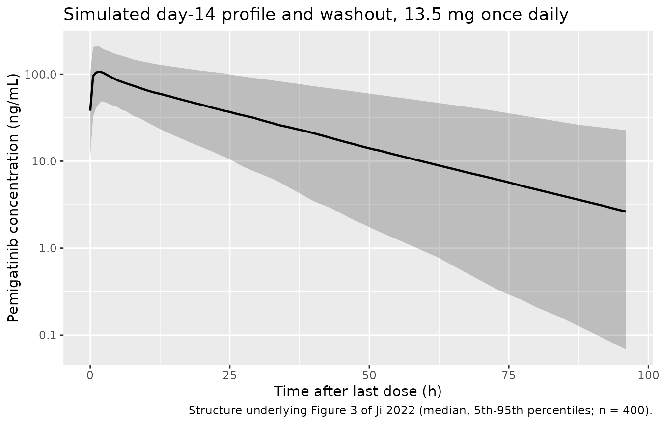
Figure 3 of Ji 2022 is a VPC of log concentration against time after the last dose for the pooled dataset (all doses and days). It cannot be reproduced exactly without the observed data and dosing history; the plot below shows the simulated median and 5th/95th percentiles at steady state (day 14, 13.5 mg once daily) followed by the washout.
sim |>
  dplyr::filter(time >= last_dose) |>
  dplyr::mutate(tad = time - last_dose) |>
  dplyr::group_by(tad) |>
  dplyr::summarise(
    Q05 = quantile(Cc, 0.05),
    Q50 = quantile(Cc, 0.50),
    Q95 = quantile(Cc, 0.95),
    .groups = "drop"
  ) |>
  ggplot(aes(tad, Q50)) +
  geom_ribbon(aes(ymin = Q05, ymax = Q95), alpha = 0.25) +
  geom_line(linewidth = 0.8) +
  scale_y_log10() +
  labs(
    x = "Time after last dose (h)", y = "Pemigatinib concentration (ng/mL)",
    title = "Simulated day-14 profile and washout, 13.5 mg once daily",
    caption = "Structure underlying Figure 3 of Ji 2022 (median, 5th-95th percentiles; n = 400)."
  )
Covariate effects on CL/F (Figure 2)
Figure 2 gives geometric mean ratios (GMRs) of the post hoc CL/F between subgroups. For the two covariates retained on CL/F, the typical-value ratio of the model is close to the post hoc GMR, as expected when the subgroups are roughly balanced on the other covariates.
fig2 <- tibble::tibble(
  Comparison = c("Female vs male", "Phosphate binder yes vs no"),
  `Model typical-value ratio` = c(
    female_nobinder$cl / male_nobinder$cl,
    male_binder$cl / male_nobinder$cl
  ),
  `Figure 2 post hoc GMR (90% CI)` = c("0.852 (0.790-0.919)", "0.872 (0.806-0.943)")
)
knitr::kable(fig2, digits = 3, caption = "Replicates the CL/F covariate rows of Figure 2A and 2C of Ji 2022.")| Comparison | Model typical-value ratio | Figure 2 post hoc GMR (90% CI) |
|---|---|---|
| Female vs male | 0.810 | 0.852 (0.790-0.919) |
| Phosphate binder yes vs no | 0.876 | 0.872 (0.806-0.943) |
PKNCA validation
conc_df <- sim |>
  dplyr::filter(!is.na(Cc)) |>
  dplyr::select(id, time, Cc, sex)

dose_df <- doses |>
  dplyr::select(id, time, amt, sex)

conc_obj <- PKNCA::PKNCAconc(conc_df, Cc ~ time | sex + id)
dose_obj <- PKNCA::PKNCAdose(dose_df, amt ~ time | sex + id)

intervals <- data.frame(
  start = c(0, last_dose, last_dose),
  end = c(tau, last_dose + tau, last_dose + 96),
  cmax = c(TRUE, TRUE, FALSE),
  tmax = c(TRUE, TRUE, FALSE),
  auclast = c(TRUE, TRUE, FALSE),
  cmin = c(FALSE, TRUE, FALSE),
  half.life = c(FALSE, FALSE, TRUE)
)

nca_res <- PKNCA::pk.nca(PKNCA::PKNCAdata(conc_obj, dose_obj, intervals = intervals))
nca_df <- as.data.frame(nca_res)

nca_df |>
  dplyr::filter(PPTESTCD %in% c("cmax", "tmax", "auclast", "cmin", "half.life")) |>
  dplyr::mutate(
    Interval = dplyr::case_when(
      start == 0 ~ "Day 1",
      end == last_dose + tau ~ "Day 14 (steady state)",
      TRUE ~ "After last dose"
    )
  ) |>
  # The washout interval requests only the half-life; drop dependency rows.
  dplyr::filter(Interval != "After last dose" | PPTESTCD == "half.life") |>
  dplyr::group_by(sex, Interval, PPTESTCD) |>
  dplyr::summarise(Median = median(PPORRES, na.rm = TRUE), .groups = "drop") |>
  tidyr::pivot_wider(names_from = PPTESTCD, values_from = Median) |>
  dplyr::rename(
    Sex = sex,
    `Cmax (ng/mL)` = cmax,
    `Tmax (h)` = tmax,
    `AUC0-24 (h*ng/mL)` = auclast,
    `Cmin (ng/mL)` = cmin,
    `t1/2 (h)` = half.life
  ) |>
knitr::kable(digits = 1, caption = "Median simulated NCA, 13.5 mg once daily.")| Sex | Interval | t1/2 (h) | AUC0-24 (h*ng/mL) | Cmax (ng/mL) | Tmax (h) | Cmin (ng/mL) |
|---|---|---|---|---|---|---|
| Female | After last dose | 20.5 | NA | NA | NA | NA |
| Female | Day 1 | NA | 950.5 | 78.0 | 1.2 | NA |
| Female | Day 14 (steady state) | NA | 1641.8 | 120.7 | 1.0 | 42.1 |
| Male | After last dose | 17.0 | NA | NA | NA | NA |
| Male | Day 1 | NA | 906.8 | 72.9 | 2.0 | NA |
| Male | Day 14 (steady state) | NA | 1459.9 | 104.8 | 1.8 | 34.7 |
Comparison against published values
Ji 2022 reports three quantities that the simulation can be compared with:
- post hoc steady-state Cmax of 156 nM (76.05 ng/mL) in men and 198 nM (96.53 ng/mL) in women (Discussion), a 27% higher Cmax,ss in women;
- a mean (SD) post hoc half-life of 16.0 (5.76) h over the evaluable population (Results);
- an accumulation ratio of about 1.6 for AUC0-24 (Introduction, from the phase 1 noncompartmental analysis).
sim_ss <- nca_df |>
  dplyr::filter(start == last_dose, end == last_dose + tau, PPTESTCD == "cmax") |>
  dplyr::select(sex, PPTESTCD, PPORRES)
sim_hl <- nca_df |>
  dplyr::filter(PPTESTCD == "half.life") |>
  dplyr::mutate(sex = "All") |>
  dplyr::select(sex, PPTESTCD, PPORRES)

ref <- data.frame(
  sex = c("Male", "Female", "All"),
  PPTESTCD = c("cmax", "cmax", "half.life"),
  PPORRES = c(76.05, 96.53, 16.0)
)

cmp <- nlmixr2lib::ncaComparisonTable(
  simulated = dplyr::bind_rows(sim_ss, sim_hl),
  reference = ref,
  by = "sex",
  units = c(cmax = "ng/mL", half.life = "h")
)
knitr::kable(cmp, caption = "Simulated (median) vs Ji 2022 reported steady-state Cmax and half-life.")| NCA parameter | sex | Reference | Simulated | % diff |
|---|---|---|---|---|
| Cmax (ng/mL) | Male | 76 | 105 | +37.9%* |
| Cmax (ng/mL) | Female | 96.5 | 121 | +25.0%* |
| t½ (h) | All | 16 | 18.8 | +17.3% |
if (!is.null(attr(cmp, "footnote"))) cat(attr(cmp, "footnote"), "\n")
#> * differs from reference by more than ±20%.

# Female / male Cmax,ss for the typical patient (73.3 kg, no binder, no PPI),
# so the sex effect is isolated from cohort sampling noise.
typ_ss <- function(SEXF) {
  ev <- rxode2::et(amt = dose_mg, ii = tau, addl = n_dose - 1, cmt = "depot") |>
    rxode2::et(seq(last_dose, last_dose + tau, by = 0.05), cmt = "central") |>
    as.data.frame()
  ev$SEXF <- SEXF
  ev$CONMED_PHOSBINDER <- 0
  ev$CONMED_PPI <- 0
  ev$WT <- 73.3
  out <- rxode2::rxSolve(rxode2::zeroRe(mod), events = ev) |> as.data.frame()
  max(out$Cc)
}
ratio_fm <- typ_ss(1) / typ_ss(0)
#> ℹ parameter labels from comments will be replaced by 'label()'
#> ℹ omega/sigma items treated as zero: 'etalcl', 'etalvc', 'etalka'
#> ℹ parameter labels from comments will be replaced by 'label()'
#> ℹ omega/sigma items treated as zero: 'etalcl', 'etalvc', 'etalka'

# Model-derived terminal half-life per simulated subject, from the individual
# micro-constants (the paper's half-life is likewise derived from post hoc
# parameters).
hl_indiv <- sim |>
  dplyr::filter(time == last_dose) |>
  dplyr::mutate(
    beta = 0.5 * ((kel + k12 + k21) - sqrt((kel + k12 + k21)^2 - 4 * kel * k21)),
    thalf = log(2) / beta
  )

# Typical-patient terminal half-life (73.3 kg, no binder, no PPI) by sex,
# from the same closed form.
thalf_typ <- function(p) {
  kel <- p$cl / p$vc
  k12 <- p$q / p$vc
  k21 <- p$q / p$vp
  log(2) / (0.5 * ((kel + k12 + k21) - sqrt((kel + k12 + k21)^2 - 4 * kel * k21)))
}
thalf_male <- thalf_typ(male_nobinder)
thalf_female <- thalf_typ(female_nobinder)

auc_d1 <- nca_df |>
  dplyr::filter(start == 0, PPTESTCD == "auclast") |>
  dplyr::select(id, auc1 = PPORRES)
auc_ss <- nca_df |>
  dplyr::filter(start == last_dose, end == last_dose + tau, PPTESTCD == "auclast") |>
  dplyr::select(id, aucss = PPORRES)
racc <- dplyr::inner_join(auc_d1, auc_ss, by = "id") |>
  dplyr::mutate(r = aucss / auc1)

knitr::kable(
  tibble::tibble(
    Quantity = c(
      "Cmax,ss female / male (typical patient)",
      "Accumulation ratio AUC0-24 (median)",
      "Terminal t1/2, typical man (h)",
      "Terminal t1/2, typical woman (h)",
      "Model-derived terminal t1/2 in the cohort, mean (h)",
      "Model-derived terminal t1/2 in the cohort, SD (h)"
    ),
    Simulated = c(
      ratio_fm, median(racc$r), thalf_male, thalf_female,
      mean(hl_indiv$thalf), sd(hl_indiv$thalf)
    ),
    Published = c(96.53 / 76.05, 1.6, 16.0, 16.0, 16.0, 5.76)
  ),
  digits = 2
)| Quantity | Simulated | Published |
|---|---|---|
| Cmax,ss female / male (typical patient) | 1.18 | 1.27 |
| Accumulation ratio AUC0-24 (median) | 1.64 | 1.60 |
| Terminal t1/2, typical man (h) | 15.22 | 16.00 |
| Terminal t1/2, typical woman (h) | 18.37 | 16.00 |
| Model-derived terminal t1/2 in the cohort, mean (h) | 19.92 | 16.00 |
| Model-derived terminal t1/2 in the cohort, SD (h) | 7.94 | 5.76 |
stopifnot(
  # Deterministic typical-value ratio vs the paper's post hoc ratio.
  abs(ratio_fm / (96.53 / 76.05) - 1) < 0.1,
  # Centre-of-distribution checks (robust to which subjects land in the tails).
  abs(median(racc$r) / 1.6 - 1) < 0.15,
  # Typical-patient half-lives bracket the published population mean.
  thalf_male < 16.0, thalf_female > 16.0,
  abs(thalf_male / 16.0 - 1) < 0.2, abs(thalf_female / 16.0 - 1) < 0.2
)
The accumulation ratio agrees with the paper, and the typical-patient half-lives (about 15 h in men and 18 h in women) bracket the published mean of 16.0 h. The cohort mean of the model-derived half-life is higher (about 20 h) and more dispersed than the published 16.0 (5.76) h; the published value summarises post hoc estimates, which are shrunk towards the typical values (shrinkage 7.6% on CL/F and 21.9% on Vc/F), while the simulation draws the full IIV. The sex effect on Cmax,ss for the typical patient (female/male about 1.18) is a little smaller than the 1.27 the paper reports from post hoc estimates, which also carry the other covariate differences between men and women in the dataset.
The absolute simulated Cmax,ss at 13.5 mg is 25-40% above the Discussion’s post hoc values (76.05 ng/mL in men, 96.53 ng/mL in women). The model was not adjusted to close this gap. The typical male CL/F of 10.27 L/h implies an AUC0-24,ss of 13.5 mg / 10.27 L/h = 1314 h*ng/mL (an average concentration of 55 ng/mL) at 13.5 mg, and with the printed ka and Vc/F the peak is about 105 ng/mL; a Cmax,ss of 76 ng/mL would need a dose near 10 mg. The paper does not say at which dose or occasion its post hoc Cmax,ss was computed. The analysis dataset mixes doses from 1 to 20 mg (FIGHT-101) and 9 mg (FIGHT-102) with 13.5 mg, so a dataset-wide summary below the 13.5 mg value is expected. The published half-life (mean 16.0 h) is likewise a summary of model-derived terminal half-lives; the PKNCA half-life in the table above is fitted over 24-96 h after the last dose.
Assumptions and deviations
-
Covariate coding. Equations I-IV are encoded as
printed. The source column SEXN (1 = male, 2 = female) is replaced by
the canonical
SEXF(1 = female) throughSEXN = 1 + SEXF. The paper’s reference levels are kept: the typical CL/F of 9.00 L/h is a man on a phosphate binder, and the typical Vc/F of 161 L is a 73.3-kg patient on a PPI. - PPI coding. The “Where:” block defines BINDER but not PPI. PPI is taken as 1 = used, 0 = not used, by analogy with BINDER; this reproduces the Results statement that Vc/F is 122.0 L at 73.3 kg (without a PPI) and the direction of the stated PPI effect.
- Time-varying co-medications. BINDER and PPI vary by visit in the source dataset; in this vignette each virtual subject is either on or off for the whole simulation.
-
Residual error. The model was fitted to
log-transformed concentrations with an additive error of SD 0.401 on the
log scale, encoded as
Cc ~ lnorm(expSd). -
Concentration units. Doses are in mg and volumes in
L, so
Cc = 1000 * central / vcis in ng/mL, matching the paper’s statement that concentrations were analysed in mass units and the ng/mL axes of Figure 1. - Virtual cohort. Body weight is log-normal around 73.3 kg (SD of log-weight 0.25, not reported); covariate prevalences are taken from Table 3 and treated as independent.
Errata and reporting gaps
- Sex labels in the Results and Abstract. The Results state “The typical pemigatinib ka and CL/F were estimated at 1.49 h-1 and 10.3 L/h, respectively, for female patients” and that for men CL/F is 19.0% higher and ka 56.5% lower. Under the printed coding SEXN = 1 male / 2 female, Equations I and IV give ka = 1.49 1/h and CL/F = 10.27 L/h (no binder) for men, and for women CL/F x 0.81 and ka x 1.565. The equations, the Discussion (“typical ka value is 56.5% higher for female patients”, “typical CL/F value of female patients is 19% lower than male patients”), the higher Cmax,ss reported for women and the Figure 2A GMR of 0.852 (female vs male) all agree with each other, so the equations are encoded as printed and the Results/Abstract sentence is treated as a sex-label slip. The later Gong 2023 analysis of the same programme estimates the same direction (higher CL/F and lower ka in men).
- Percent effects in the text (“phosphate binders decrease CL/F by 14.1%”, “PPI increases Vc/F by 24.4%”) quote the coefficients rather than the implied changes. With the printed equations, binder use lowers CL/F by 1 - 1/1.141 = 12.4% and PPI use raises Vc/F by 1/0.756 - 1 = 32.3%.
- Sex effect on ka (0.565) appears in Equation IV and the Results text but has no row in Table 4.
- Geometric mean CL/F of 10.9 L/h (Discussion) is not reproducible from the final model: the largest typical CL/F the equations allow (a man not on a phosphate binder) is 10.27 L/h, and the covariate mix of Tables 2-3 gives a typical value near 8.7 L/h. The figure is close to the base-model CL/F of 10.7 L/h and may come from an intermediate model.
- Figure axes. Figures 1 and 3 label the concentration axis “log of ng/mL”, but the plotted values (up to about 6.7 on the log scale, above the 488 ng/mL upper limit of quantitation) would fit the nM scale better (1000 nM ULOQ). This affects only how the figures are read; the fitted CL/F agrees with the noncompartmental CL/F of 9.88-11.7 L/h cited in the Discussion, so the parameters are on the physical mg and L scale.