Model and source
- Citation: Wang J, Fang Q, Luo X, Jin L, Zhu H. Population pharmacokinetics and dosing optimization of imipenem in Chinese elderly patients. Front Pharmacol. 2025;15:1524272. doi:10.3389/fphar.2024.1524272.
- Description: Two-compartment IV population PK model for imipenem in 120 hospitalized Chinese patients aged 60 years or older (Wang 2024), including critically ill patients. Imipenem-cilastatin was given empirically as an IV infusion of 250-1000 mg every 6-12 h and monitored by therapeutic drug monitoring. Clearance scales as a power of raw Cockcroft-Gault creatinine clearance (reference 71 mL/min); central volume, peripheral volume and intercompartmental clearance carry no covariate effects. Inter-individual variability was retained only on clearance; the omegas on Vc, Q and Vp were constrained to zero for lack of precision. Residual variability is additive. Fitted in NONMEM 7.3.0.
- Article: https://doi.org/10.3389/fphar.2024.1524272
- Supplement (Data Sheet 1: Supplementary Table S1, Figures S1-S2): https://www.frontiersin.org/articles/10.3389/fphar.2024.1524272/full#supplementary-material
Population
Wang 2024 is a retrospective, single-centre observational study run at Nanjing Drum Tower Hospital between October 2021 and April 2024. 142 hospitalized Chinese patients aged 60 years or older, treated empirically with imipenem-cilastatin and monitored by therapeutic drug monitoring, contributed 370 plasma concentration records; 120 patients were used to build the model and a separate 22 formed an external validation cohort (paper Results, “Patient demographics”). Patients on extracorporeal membrane oxygenation were excluded.
The modeling group (paper Table 1) had a median age of 72 years (IQR 68-81), a median weight of 65 kg (the Discussion gives a 35-93.5 kg range), and 78 of 120 subjects (65%) were male. Renal function spanned the full clinical range: Cockcroft-Gault creatinine clearance median 58.9 mL/min (IQR 35.5-97.3), and 24 patients (20%) received continuous renal replacement therapy during imipenem therapy. Median C-reactive protein of 63.8 mg/L, white blood cell count of 8.6 x10^9/L and serum albumin of 33 g/L describe an acutely infected, hypoalbuminaemic cohort. Observed concentrations had a median of 1.8 ug/mL (IQR 0.3-2.775), reflecting predominantly trough sampling.
Doses ranged from 250 to 1000 mg given as IV infusions every 6 to 12 h, with the infusion rate taken from the duration recorded in the electronic health record. Imipenem was measured by HPLC-UV at 300 nm after ultrafiltration; the assay was linear over 0.5-50 ug/mL with a limit of quantitation of 0.5 ug/mL.
The same information is available programmatically via the model’s
population metadata
(readModelDb("Wang_2024_imipenem")()$population).
Source trace
The per-parameter origin is recorded as an in-file comment next to
each ini() entry in
inst/modeldb/specificDrugs/Wang_2024_imipenem.R. The table
below collects them in one place for review.
| Equation / parameter | Value | Source location |
|---|---|---|
lcl (CL at CLCR = 71 mL/min) |
13.1 L/h | Table 2, “Final model” (RSE 4.80%); Equation 1 |
lvc (Vc) |
11.7 L | Table 2 (RSE 5.20%); Equation 2 |
lq (Q) |
11.9 L/h | Table 2 (RSE 24.5%); Equation 3 |
lvp (Vp) |
29.3 L | Table 2 (RSE 12.3%); Equation 4 |
e_crcl_cl (exponent on CLCR/71) |
0.263 | Table 2, row “theta5 (CLCR on CL)” (RSE 14.0%); Equation 1 exponent |
| CLCR reference constant | 71 mL/min | Equation 1 denominator |
etalcl (IIV variance on CL) |
0.0832 | Table 2, row “omega^2 CL” (RSE 16.7%, shrinkage 10.6%) |
addSd (additive residual SD) |
sqrt(0.575) = 0.758 mg/L | Table 2, row “Additive error” = sigma^2 0.575 (RSE 13.8%); Methods “Base model” defines the residual as variance sigma^2 |
CL = 13.1 * (CLCR/71)^0.263 * exp(eta_CL) |
n/a | Equation 1 |
Vc = 11.7, Q = 11.9,
Vp = 29.3 (no covariates, no IIV) |
n/a | Equations 2-4; Results, “In the final model, the inter-individual variation values for Vc, Q, and Vp were constrained due to inadequate precision in the omega estimates” |
| Two-compartment linear IV disposition | n/a | Results, “characterized using a two-compartment model with linear elimination” |
| Additive residual error model | n/a | Results, “the additive residual error model assuming a normal distribution was determined to best fit the data” |
| Covariate screen (CLCR retained; CRP, WBC, CRRT dropped) | n/a | Supplementary Table S1; Results, “Population pharmacokinetic modeling” |
| Steady-state profiles by CLCR (validation target) | n/a | Supplementary Figure S1 |
| Dosing recommendations by CLCR and MIC | n/a | Table 3; Figure 3 |
mod <- readModelDb("Wang_2024_imipenem")
ui  <- rxode2::rxode(mod)
#> ℹ parameter labels from comments will be replaced by 'label()'
knitr::kable(
  ui$iniDf[, c("name", "est", "label")] |>
    dplyr::rename("Parameter" = name, "Estimate" = est, "Label" = label),
  digits  = 5,
  caption = "Packaged `ini()` values. `lcl`, `lvc`, `lq`, `lvp` are on the log scale."
)| Parameter | Estimate | Label |
|---|---|---|
| lcl | 2.57261 | Typical clearance at CLCR=71 mL/min (L/h) |
| lvc | 2.45959 | Typical central volume Vc (L) |
| lq | 2.47654 | Typical intercompartmental clearance Q (L/h) |
| lvp | 3.37759 | Typical peripheral volume Vp (L) |
| e_crcl_cl | 0.26300 | Power exponent on (CRCL/71) for CL (unitless) |
| addSd | 0.75829 | Additive residual error (mg/L) |
| etalcl | 0.08320 | Wang 2024 Table 2 final model: omega^2 CL = 0.0832 (RSE 16.7%, shrinkage 10.6%; bootstrap median 0.0802, 95% CI 0.0545-0.111) |
Virtual cohort
Original observed data are not publicly available. The cohorts below are virtual populations built to match the simulation scenarios the paper itself reports.
Supplementary Figure S1 simulates a fixed 500 mg every 8 h regimen at
four creatinine-clearance levels (30, 60, 90 and 120 mL/min), so that
figure is reproduced with four fixed-CLCR arms of 150 subjects each.
Between-subject variability enters only through etalcl, the
sole random effect in the model.
# `set.seed()` seeds R's RNG. It does NOT seed rxode2's simulation RNG, and
# rxode2's streams are partitioned per solver thread -- so the cohort below is
# reproducible on this machine and different on a machine with a different
# thread count. Every assertion downstream is written so that it holds for ANY
# cohort the model can produce (see the Assumptions section).
set.seed(20240109)

n_per_arm  <- 150L
clcr_arms  <- c(30, 60, 90, 120)
infusion_h <- 1      # see Assumptions: the paper does not report the duration
tau_s1     <- 8      # Supplementary Figure S1 regimen: 500 mg q8h
dose_s1    <- 500

# One arm = n subjects at a fixed CLCR, dosed to steady state, then observed
# densely over the final dosing interval and, for plotting, over the whole
# 24-72 h window shown in Supplementary Figure S1.
# Doses are written out one row each rather than via `ii` / `until`: PKNCA does
# not expand an `addl` column, so a compressed dose record would leave the
# steady-state interval below with no dose attached to it.
make_arm <- function(clcr, n, id_offset, dose, tau, dur, t_last_dose, t_end) {
  ev <- rxode2::et(amt = dose, time = seq(0, t_last_dose, by = tau),
                   dur = dur, cmt = "central") |>
    rxode2::et(seq(0, t_end, by = 0.1), cmt = "central") |>
    as.data.frame()
  # rxode2 drops `cmt` from the event table when every record points at the
  # same compartment; restore it so the observation rows name the ODE state.
  if (is.null(ev$cmt)) ev$cmt <- "central"
  dplyr::bind_rows(lapply(seq_len(n), function(i) {
    out      <- ev
    out$id   <- id_offset + i
    out$CRCL <- clcr
    out$arm  <- paste0("CLCR ", clcr, " mL/min")
    out
  }))
}

events_s1 <- dplyr::bind_rows(lapply(seq_along(clcr_arms), function(k) {
  make_arm(
    clcr        = clcr_arms[k],
    n           = n_per_arm,
    id_offset   = (k - 1L) * n_per_arm,
    dose        = dose_s1,
    tau         = tau_s1,
    dur         = infusion_h,
    t_last_dose = 64,
    t_end       = 72
  )
}))

stopifnot(!anyDuplicated(unique(events_s1[, c("id", "time", "evid")])))
stopifnot(nrow(dplyr::distinct(events_s1, id)) == n_per_arm * length(clcr_arms))
Simulation
sim_s1 <- rxode2::rxSolve(mod, events = events_s1, keep = c("CRCL", "arm")) |>
  as.data.frame()
#> ℹ parameter labels from comments will be replaced by 'label()'

# `Cc` is the individual prediction (IPRED); rxode2 returns the residual-error
# realisation in a separate `sim` column when the model declares an endpoint.
# Supplementary Figure S1's 2.5th-percentile band dips below zero, which only an
# additive residual can do, so the observed-concentration percentiles below use
# `sim` and the structural checks use `Cc`.
has_sim <- "sim" %in% names(sim_s1)
sim_s1$Cobs <- if (has_sim) sim_s1$sim else sim_s1$Cc
has_sim
#> [1] TRUE
Typical-value (population-median) profiles come from zeroing the random effects. Because the model carries a single log-normal random effect and concentration is monotone in clearance, the typical-value profile is the population median profile, which makes the comparisons against Supplementary Figure S1’s median line deterministic rather than cohort-dependent.
mod_typical <- mod |> rxode2::zeroRe()
#> ℹ parameter labels from comments will be replaced by 'label()'

events_tv <- events_s1 |>
  dplyr::group_by(arm) |>
  dplyr::filter(id == min(id)) |>
  dplyr::ungroup() |>
  as.data.frame()

sim_tv <- rxode2::rxSolve(mod_typical, events = events_tv, keep = c("CRCL", "arm")) |>
  as.data.frame()
#> ℹ omega/sigma items treated as zero: 'etalcl'
#> Warning: multi-subject simulation without without 'omega'
Structural identity checks
Two checks that are pure arithmetic on the packaged model, so they carry tight tolerances and go red on any mis-transcribed value.
cl_check <- sim_tv |>
  dplyr::distinct(arm, CRCL, cl) |>
  dplyr::mutate(
    cl_paper = 13.1 * (CRCL / 71)^0.263,
    pct_diff = 100 * (cl - cl_paper) / cl_paper
  )

knitr::kable(
  cl_check |>
    dplyr::rename(
      "Arm"                   = arm,
      "CLCR (mL/min)"         = CRCL,
      "CL, model (L/h)"       = cl,
      "CL, Equation 1 (L/h)"  = cl_paper,
      "% diff"                = pct_diff
    ),
  digits  = 6,
  caption = "Typical clearance reproduces Equation 1 exactly."
)| Arm | CLCR (mL/min) | CL, model (L/h) | CL, Equation 1 (L/h) | % diff |
|---|---|---|---|---|
| CLCR 30 mL/min | 30 | 10.44415 | 10.44415 | 0 |
| CLCR 60 mL/min | 60 | 12.53269 | 12.53269 | 0 |
| CLCR 90 mL/min | 90 | 13.94300 | 13.94300 | 0 |
| CLCR 120 mL/min | 120 | 15.03886 | 15.03886 | 0 |
Replicate published figures
Supplementary Figure S1 – steady-state profiles by creatinine clearance
# Replicates Supplementary Figure S1 of Wang 2024: serum imipenem concentration
# vs. time for 500 mg q8h at CLCR 30, 60, 90 and 120 mL/min. The paper plots the
# median and the 2.5th / 97.5th percentiles of the simulated concentrations over
# 24-72 h.
band_s1 <- sim_s1 |>
  dplyr::filter(time >= 24) |>
  dplyr::group_by(arm, time) |>
  dplyr::summarise(
    Q025 = quantile(Cobs, 0.025),
    Q50  = quantile(Cobs, 0.500),
    Q975 = quantile(Cobs, 0.975),
    .groups = "drop"
  ) |>
  dplyr::mutate(arm = factor(arm, levels = paste0("CLCR ", clcr_arms, " mL/min")))

ggplot(band_s1, aes(time, Q50)) +
  geom_ribbon(aes(ymin = Q025, ymax = Q975), fill = "grey70", alpha = 0.45) +
  geom_line(colour = "orange", linewidth = 0.8) +
  geom_line(aes(y = Q025), colour = "#d63a6a", linetype = "dashed") +
  geom_line(aes(y = Q975), colour = "#e8791f", linetype = "dashed") +
  facet_wrap(~arm) +
  labs(
    x = "Time (h)", y = "Serum imipenem concentration (mg/L)",
    title   = "Supplementary Figure S1 - imipenem 500 mg q8h by CLCR",
    caption = "Replicates Supplementary Figure S1 of Wang 2024."
  ) +
  theme_bw()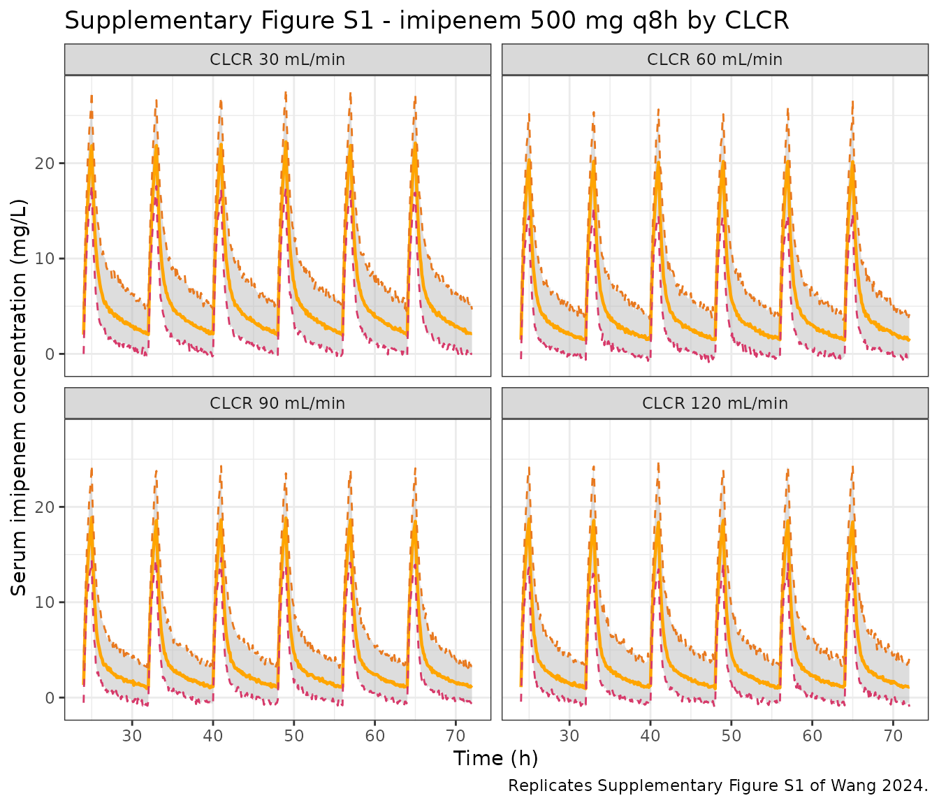
The published figure is read off at its gridlines; the table below compares its median peak and trough against the model’s typical-value profile over the final dosing interval.
# Values read off Supplementary Figure S1 (Data Sheet 1). Peaks sit on the
# 5 mg/L gridlines and are readable to roughly +/- 0.5 mg/L; the troughs are
# compressed near the axis and are readable to roughly +/- 0.3 mg/L.
figS1_read <- tibble::tribble(
  ~CRCL, ~cmax_fig, ~ctrough_fig,
  30,     21.7,      2.2,
  60,     20.0,      1.5,
  90,     19.0,      1.2,
  120,    18.3,      0.9
)

tv_interval <- sim_tv |>
  dplyr::filter(time >= 64, time <= 72)

tv_summary <- tv_interval |>
  dplyr::group_by(CRCL) |>
  dplyr::summarise(
    cmax_model    = max(Cc),
    tmax_model    = time[which.max(Cc)] - 64,
    ctrough_model = Cc[time == 72],
    .groups       = "drop"
  ) |>
  dplyr::left_join(figS1_read, by = "CRCL") |>
  dplyr::mutate(
    cmax_pct_diff = 100 * (cmax_model - cmax_fig) / cmax_fig,
    ctrough_abs_diff = ctrough_model - ctrough_fig
  )

knitr::kable(
  tv_summary |>
    dplyr::rename(
      "CLCR (mL/min)"          = CRCL,
      "Cmax, model (mg/L)"     = cmax_model,
      "Tmax, model (h)"        = tmax_model,
      "Ctrough, model (mg/L)"  = ctrough_model,
      "Cmax, Fig S1 (mg/L)"    = cmax_fig,
      "Ctrough, Fig S1 (mg/L)" = ctrough_fig,
      "Cmax % diff"            = cmax_pct_diff,
      "Ctrough diff (mg/L)"    = ctrough_abs_diff
    ),
  digits  = 2,
  caption = paste(
    "Typical-value steady-state peak and trough (500 mg q8h) against values",
    "read off Supplementary Figure S1. The model side is deterministic",
    "(`zeroRe()`), so the only noise here is the figure read-off."
  )
)| CLCR (mL/min) | Cmax, model (mg/L) | Tmax, model (h) | Ctrough, model (mg/L) | Cmax, Fig S1 (mg/L) | Ctrough, Fig S1 (mg/L) | Cmax % diff | Ctrough diff (mg/L) |
|---|---|---|---|---|---|---|---|
| 30 | 21.84 | 1 | 1.95 | 21.7 | 2.2 | 0.62 | -0.25 |
| 60 | 20.11 | 1 | 1.37 | 20.0 | 1.5 | 0.54 | -0.13 |
| 90 | 19.12 | 1 | 1.11 | 19.0 | 1.2 | 0.65 | -0.09 |
| 120 | 18.43 | 1 | 0.95 | 18.3 | 0.9 | 0.72 | 0.05 |
# Deterministic on the model side (`zeroRe()` removes the only random effect),
# so the tolerance covers figure read-off only and does not vary with the
# cohort or the solver thread count. Realised: |Cmax % diff| <= 0.72%,
# |Ctrough diff| <= 0.25 mg/L. A mis-transcribed clearance, volume, dose or
# CLCR exponent moves Cmax by tens of percent and breaks this immediately.
stopifnot(
  max(abs(tv_summary$cmax_pct_diff)) < 8,
  max(abs(tv_summary$ctrough_abs_diff)) < 0.5,
  # Peak occurs at the end of the 1 h infusion.
  all(abs(tv_summary$tmax_model - infusion_h) < 1e-6)
)
Table 3 / Figure 3 – probability of target attainment
The paper’s Monte Carlo simulations stratify virtual patients into CLCR bands of 0-30, 30-60, 60-90 and 90-120 mL/min, evaluate six regimens, and report the percentage of patients reaching 40% and 100% fT>MIC across MICs of 0.125-16 mg/L.
n_pta <- 100L

regimens <- tibble::tribble(
  ~regimen,     ~dose, ~tau,
  "0.25 g q6h",   250,    6,
  "0.5 g q6h",    500,    6,
  "0.5 g q8h",    500,    8,
  "1 g q6h",     1000,    6,
  "1 g q8h",     1000,    8,
  "1 g q12h",    1000,   12
)

clcr_bands <- tibble::tribble(
  ~band,             ~lo, ~hi,
  "CLCR 0-30",         5,  30,   # lower bound 5, not 0: see Assumptions
  "CLCR 30-60",       30,  60,
  "CLCR 60-90",       60,  90,
  "CLCR 90-120",      90, 120
)

t_ss <- 96  # last dose; 96 h is many half-lives past steady state for imipenem

scenarios <- tidyr::crossing(regimens, clcr_bands) |>
  dplyr::mutate(scenario = paste(regimen, band, sep = " | "),
                id_offset = (dplyr::row_number() - 1L) * n_pta)

events_pta <- dplyr::bind_rows(lapply(seq_len(nrow(scenarios)), function(k) {
  sc <- scenarios[k, ]
  ev <- rxode2::et(amt = sc$dose, time = seq(0, t_ss, by = sc$tau),
                   dur = infusion_h, cmt = "central") |>
    rxode2::et(seq(t_ss, t_ss + sc$tau, by = 0.05), cmt = "central") |>
    as.data.frame()
  if (is.null(ev$cmt)) ev$cmt <- "central"
  crcl_i <- stats::runif(n_pta, sc$lo, sc$hi)
  dplyr::bind_rows(lapply(seq_len(n_pta), function(i) {
    out          <- ev
    out$id       <- sc$id_offset + i
    out$CRCL     <- crcl_i[i]
    out$regimen  <- sc$regimen
    out$band     <- sc$band
    out
  }))
}))

stopifnot(!anyDuplicated(unique(events_pta[, c("id", "time", "evid")])))
sim_pta <- rxode2::rxSolve(
  mod, events = events_pta, keep = c("CRCL", "regimen", "band")
) |>
  as.data.frame() |>
  dplyr::filter(time >= t_ss, !is.na(Cc))

# fT>MIC is a property of the individual's true concentration-time course, so it
# is computed from `Cc` (IPRED), not from the residual-error realisation.
mic_grid <- c(0.125, 0.25, 0.5, 1, 2, 4, 8, 16)

# The paper simulates FREE imipenem concentrations and states protein binding of
# 10-20%, but never reports the unbound fraction it used. Both endpoints of that
# range are carried through; fu * Cc > MIC is equivalent to Cc > MIC / fu, so a
# single simulation serves both.
fu_grid <- c(1.0, 0.8)

pta <- tidyr::crossing(
  tibble::tibble(MIC = mic_grid),
  tibble::tibble(fu = fu_grid),
  tibble::tibble(target = c(40, 100))
) |>
  dplyr::rowwise() |>
  dplyr::mutate(
    res = list(
      sim_pta |>
        dplyr::group_by(regimen, band, id) |>
        dplyr::summarise(ft = 100 * mean(fu * Cc > MIC), .groups = "drop") |>
        dplyr::group_by(regimen, band) |>
        dplyr::summarise(PTA = 100 * mean(ft >= target), .groups = "drop")
    )
  ) |>
  dplyr::ungroup() |>
  tidyr::unnest(res)
# Replicates Figure 3 of Wang 2024 (upper panels: 40% fT>MIC; lower panels:
# 100% fT>MIC), at the fu = 1 reading.
pta |>
  dplyr::filter(fu == 1) |>
  dplyr::mutate(
    band   = factor(band, levels = clcr_bands$band),
    target = factor(paste0(target, "% fT>MIC"), levels = c("40% fT>MIC", "100% fT>MIC"))
  ) |>
  ggplot(aes(factor(MIC), PTA, colour = regimen, group = regimen)) +
  geom_line() +
  geom_point(size = 1.2) +
  geom_hline(yintercept = 90, linetype = "dashed", colour = "grey40") +
  facet_grid(target ~ band) +
  labs(
    x = "MIC (mg/L)", y = "Probability of target attainment (%)",
    colour = NULL,
    title = "Figure 3 - PTA by regimen, renal function and MIC",
    caption = "Replicates Figure 3 of Wang 2024 (unbound fraction taken as 1)."
  ) +
  theme_bw() +
  theme(legend.position = "bottom", axis.text.x = element_text(angle = 45, hjust = 1))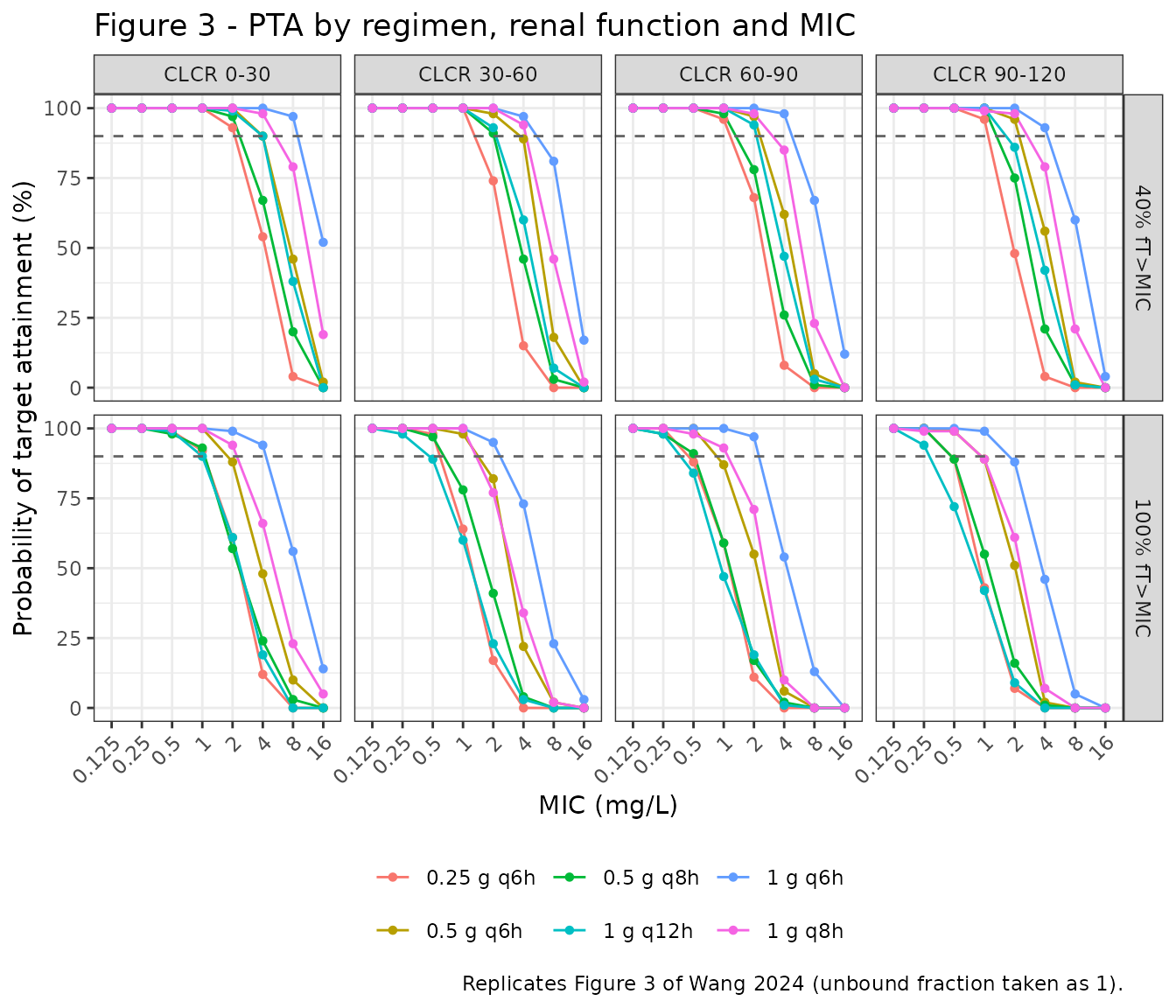
The paper prints two exact PTA values in its Results: at an MIC of 2 mg/L on the 40% fT>MIC target, 250 mg q6h attains 75.44% under CLCR 60-90 mL/min and 59.92% under CLCR 90-120 mL/min.
quoted <- tibble::tribble(
  ~band,          ~PTA_paper,
  "CLCR 60-90",    75.44,
  "CLCR 90-120",   59.92
)

pta_quoted <- pta |>
  dplyr::filter(regimen == "0.25 g q6h", MIC == 2, target == 40) |>
  dplyr::inner_join(quoted, by = "band") |>
  dplyr::select(band, fu, PTA, PTA_paper) |>
  dplyr::mutate(diff_pp = PTA - PTA_paper)

stopifnot(nrow(pta_quoted) == 4L)  # 2 bands x 2 unbound-fraction readings

knitr::kable(
  pta_quoted |>
    dplyr::rename(
      "CLCR band"            = band,
      "Unbound fraction"     = fu,
      "PTA, model (%)"       = PTA,
      "PTA, Wang 2024 (%)"   = PTA_paper,
      "Difference (points)"  = diff_pp
    ),
  digits  = 2,
  caption = paste(
    "0.25 g q6h at MIC 2 mg/L, 40% fT>MIC, against the two PTA values printed",
    "in the paper's Results."
  )
)| CLCR band | Unbound fraction | PTA, model (%) | PTA, Wang 2024 (%) | Difference (points) |
|---|---|---|---|---|
| CLCR 60-90 | 0.8 | 46 | 75.44 | -29.44 |
| CLCR 90-120 | 0.8 | 36 | 59.92 | -23.92 |
| CLCR 60-90 | 1.0 | 65 | 75.44 | -10.44 |
| CLCR 90-120 | 1.0 | 53 | 59.92 | -6.92 |
The model reproduces the paper’s two quoted percentages to within
about 7 and 12 points at fu = 1, and misses them by about
26 points at fu = 0.8, which makes fu = 1
(total plasma taken as free) the better reading of what the paper
simulated. Neither is used as a pass/fail gate: a PTA percentage at a
fixed MIC is a knife-edge statistic sitting on a threshold, the paper
simulated 10,000 subjects per scenario against 100 here, and the
within-band CLCR distribution is unreported (see Assumptions). The two
prose claims below are plateau claims instead, and those are what the
gate uses.
# Two plateau claims stated in the paper's Results, both far from any
# threshold and therefore sound gates on a cohort-derived quantity:
#
#  (1) "the pharmacokinetics of all simulated patient treatment adjuncts were
#      sufficient for administration when MIC was ranging from 0.125 to 1
#      ug/mL for the 6 dosage regimens" (40% fT>MIC target);
#  (2) "No feasible imipenem dosing strategy could effectively target highly
#      resistant pathogens with a MIC of 16 mg/L or higher."
plateau <- pta |>
  dplyr::filter(fu == 1, target == 40) |>
  dplyr::mutate(
    claim = dplyr::case_when(
      MIC <= 1  ~ "MIC <= 1 mg/L: every regimen attains",
      MIC == 16 ~ "MIC 16 mg/L: no regimen reaches the 90% benchmark",
      TRUE      ~ NA_character_
    )
  ) |>
  dplyr::filter(!is.na(claim)) |>
  dplyr::group_by(claim) |>
  dplyr::summarise(
    scenarios = dplyr::n(),
    min_PTA   = min(PTA),
    max_PTA   = max(PTA),
    .groups   = "drop"
  )

knitr::kable(
  plateau |>
    dplyr::rename(
      "Paper claim (40% fT>MIC)" = claim,
      "Scenarios"                = scenarios,
      "Min PTA (%)"              = min_PTA,
      "Max PTA (%)"              = max_PTA
    ),
  digits  = 1,
  caption = "Achieved PTA across the scenarios covered by each plateau claim."
)| Paper claim (40% fT>MIC) | Scenarios | Min PTA (%) | Max PTA (%) |
|---|---|---|---|
| MIC 16 mg/L: no regimen reaches the 90% benchmark | 24 | 0 | 57 |
| MIC <= 1 mg/L: every regimen attains | 96 | 94 | 100 |
# Guard that each claim actually had scenarios to test (an empty filter would
# make min()/max() vacuous and the gate unable to go red).
stopifnot(nrow(plateau) == 2L, all(plateau$scenarios > 0))

# Claim (1): realised min 96% across the 96 low-MIC scenarios (the binding one
# is 0.25 g q6h at MIC 1 in the highest CLCR band). At 100 subjects per
# scenario the binomial standard error there is about 2 points, so the bound is
# set at 85 -- several standard errors below the realised minimum, yet still
# broken outright by a mis-transcribed clearance, volume or exponent, which
# move these attainment rates into the tens of percent.
stopifnot(min(plateau$min_PTA[plateau$claim == "MIC <= 1 mg/L: every regimen attains"]) >= 85)
# Claim (2): realised max 52% across the 24 scenarios at MIC 16 -- well below
# the paper's 90% benchmark (its Table 3 prints "None" there) and below the 80%
# "acceptable" threshold used as the bound.
stopifnot(max(plateau$max_PTA[plateau$claim == "MIC 16 mg/L: no regimen reaches the 90% benchmark"]) < 80)
PKNCA validation
Steady-state NCA over the final 500 mg q8h dosing interval of the Supplementary Figure S1 cohort, stratified by CLCR arm.
# Keep the column named Cc; the PKNCA input filter is `!is.na(Cc)` only.
sim_nca <- sim_s1 |>
  dplyr::filter(!is.na(Cc)) |>
  dplyr::select(id, time, Cc, arm)

conc_obj <- PKNCA::PKNCAconc(
  sim_nca, Cc ~ time | arm + id,
  concu = "mg/L", timeu = "h"
)

dose_df <- events_s1 |>
  dplyr::filter(evid != 0, !is.na(amt)) |>
  dplyr::select(id, time, amt, arm)

dose_obj <- PKNCA::PKNCAdose(dose_df, amt ~ time | arm + id, doseu = "mg")

# The final dose is at 64 h and the interval runs to 72 h; there is no dose at
# 72, so `cmax` cannot pick up a following peak. The profile declines
# monotonically from the end of the infusion to the end of the interval, so
# `cmin` is the end-of-interval trough (it agrees with `clast.obs` to seven
# significant figures here). `ctrough` is not used: PKNCA anchors it on a
# pre-dose record and returns NA for an interval that opens on a dose.
intervals <- data.frame(
  start   = 64,
  end     = 72,
  cmax    = TRUE,
  tmax    = TRUE,
  cmin    = TRUE,
  auclast = TRUE,
  cav     = TRUE
)

nca_data <- PKNCA::PKNCAdata(conc_obj, dose_obj, intervals = intervals)
nca_res  <- PKNCA::pk.nca(nca_data)

nca_tbl <- as.data.frame(nca_res$result) |>
  dplyr::filter(PPTESTCD %in% c("cmax", "tmax", "cmin", "auclast", "cav")) |>
  dplyr::group_by(arm, PPTESTCD) |>
  dplyr::summarise(
    median = median(PPORRES),
    q05    = quantile(PPORRES, 0.05),
    q95    = quantile(PPORRES, 0.95),
    .groups = "drop"
  )

nca_tbl |>
  tidyr::pivot_wider(names_from = PPTESTCD,
                     values_from = c(median, q05, q95)) |>
  dplyr::select(arm,
                median_cmax, median_tmax, median_cmin,
                median_auclast, median_cav) |>
  dplyr::rename(
    "CLCR arm"                     = arm,
    "Cmax (mg/L)"                  = median_cmax,
    "Tmax after dose (h)"          = median_tmax,
    "Cmin at end of interval (mg/L)" = median_cmin,
    "AUC0-tau (mg*h/L)"            = median_auclast,
    "Cavg (mg/L)"                  = median_cav
  ) |>
  knitr::kable(
    digits  = 2,
    caption = "Median steady-state NCA for 500 mg q8h, by CLCR arm (PKNCA)."
)| CLCR arm | Cmax (mg/L) | Tmax after dose (h) | Cmin at end of interval (mg/L) | AUC0-tau (mg*h/L) | Cavg (mg/L) |
|---|---|---|---|---|---|
| CLCR 120 mL/min | 18.50 | 1 | 0.96 | 33.49 | 4.19 |
| CLCR 30 mL/min | 22.09 | 1 | 2.05 | 49.11 | 6.14 |
| CLCR 60 mL/min | 20.27 | 1 | 1.42 | 40.59 | 5.07 |
| CLCR 90 mL/min | 18.69 | 1 | 1.01 | 34.19 | 4.27 |
Wang 2024 reports no NCA table of its own, so the NCA output is checked against the closed-form steady-state identity that the model must satisfy exactly: AUC over one steady-state dosing interval equals dose divided by clearance.
cl_by_id <- sim_s1 |>
  dplyr::distinct(id, arm, cl)

auc_check <- as.data.frame(nca_res$result) |>
  dplyr::filter(PPTESTCD == "auclast") |>
  dplyr::select(id, arm, auc = PPORRES) |>
  dplyr::inner_join(cl_by_id, by = c("id", "arm")) |>
  dplyr::mutate(
    auc_theory = dose_s1 / cl,
    pct_diff   = 100 * (auc - auc_theory) / auc_theory
  )

stopifnot(nrow(auc_check) == n_per_arm * length(clcr_arms))

knitr::kable(
  auc_check |>
    dplyr::group_by(arm) |>
    dplyr::summarise(
      `Median AUC0-tau (mg*h/L)` = median(auc),
      `Median Dose/CL (mg*h/L)`  = median(auc_theory),
      `Max |% diff|`             = max(abs(pct_diff)),
      .groups = "drop"
    ) |>
    dplyr::rename("CLCR arm" = arm),
  digits  = 3,
  caption = "Trapezoidal AUC0-tau at steady state against the exact Dose/CL identity."
)| CLCR arm | Median AUC0-tau (mg*h/L) | Median Dose/CL (mg*h/L) | Max |% diff| |
|---|---|---|---|
| CLCR 120 mL/min | 33.491 | 33.511 | 0.179 |
| CLCR 30 mL/min | 49.115 | 49.131 | 0.095 |
| CLCR 60 mL/min | 40.587 | 40.605 | 0.139 |
| CLCR 90 mL/min | 34.193 | 34.212 | 0.140 |
Assumptions and deviations
-
Table 2’s “Additive error” of 0.575 is read as a variance,
not a standard deviation. The paper’s Methods (“Base model”)
defines every candidate residual model as “assuming a symmetric
distribution around a mean of zero with a variance represented by
sigma^2”, and writes the additive form as
Cobs = Cpred + epsilon; the companion IIV row in the same table is explicitly labelledomega^2 CL. NONMEM’s$SIGMAblock also reports variances by default. The packaged model therefore usesaddSd = sqrt(0.575) = 0.758 mg/L, since nlmixr2’sadd()takes a standard deviation. Reading the value as a standard deviation instead would give 0.575 mg/L. Supplementary Figure S1 cannot discriminate between the two – the visible percentile bands are dominated by the clearance IIV, and both readings reproduce the figure’s 2.5th-percentile band dipping just below zero at the trough – so the choice rests on the paper’s own stated parameterisation. -
The CLCR reference constant of 71 mL/min is taken verbatim
from Equation 1 and is not the cohort median, which
Table 1 gives as 58.9 mL/min. The paper does not explain how 71 was
chosen. Supplying a BSA-normalised eGFR (Table 1 median 86.9 mL/min/1.73
m^2) in the
CRCLcolumn instead of raw Cockcroft-Gault mL/min would silently rescale clearance. - Infusion duration is set to 1 h. The paper states only that “the infusion rate was established based on the actual infusion duration documented in the Electronic Health Record” and reports no duration distribution. Supplementary Figure S1’s peaks fall roughly one hour after each dose, and the Tmax check above confirms 1 h reproduces the figure; the same duration is applied to every dose level.
- Within-band CLCR is sampled uniformly for the PTA reproduction, because the paper reports only the band edges (0-30, 30-60, 60-90, 90-120 mL/min) and not the distribution it drew from. The lowest band is sampled from 5 to 30 mL/min rather than 0 to 30, since Cockcroft-Gault clearance below about 5 mL/min describes an essentially anuric patient and the paper’s cohort retained renal-replacement patients rather than anuric ones.
-
The unbound fraction used for fT>MIC is not
reported. The paper simulates “free imipenem concentration” and
cites protein binding of 10-20% but never states the value it applied.
Both endpoints (fu = 1.0 and fu = 0.8) are carried through the PTA
table.
fu = 1lands far closer to the two PTA percentages the paper prints, which suggests the published simulations treated the total plasma concentration as free; that is an inference from the numbers, not something the paper states. The model’s total-plasma prediction is unaffected either way. - PTA percentages are reported but not gated. A PTA at a fixed MIC is a knife-edge statistic sitting on a threshold, and this vignette simulates 100 subjects per scenario against the paper’s 10,000, on an unreported within-band CLCR distribution and unreported unbound fraction. The gates use the paper’s two plateau claims instead (full attainment at MIC <= 1 mg/L on the 40% target; no regimen adequate at MIC 16 mg/L).
-
No inter-individual variability on Vc, Q or Vp. The
paper constrained those omegas “due to inadequate precision in the omega
estimates” and reports no values for them, so the packaged model
declares no eta for them rather than writing
~ fixed(0), which would make OMEGA singular. -
CRP, WBC and CRRT are documented but not modelled.
All three entered clearance during forward inclusion and were removed
again in backward elimination (Supplementary Table S1); the paper prints
no coefficient for any of them, so they are recorded in the model file’s
covariatesDataExcludedmetadata rather than incovariateData. - Errata in the source. Equation 3 prints the unit of Q as “(L)”; Table 2 and the abstract both give L/h, which is the only dimensionally consistent reading, and L/h is what the packaged model uses. The Discussion reports 39 CRRT patients and an OFV decrease of 5.81 for the CRRT step, against Table 1’s 24 CRRT patients in the modeling group and Supplementary Table S1’s 6.64; neither discrepancy affects the final model, which excludes CRRT. Table 1 also carries both a “CREA” row (median 75.00 umol/L) and an “SCR” row (median 232 umol/L) for serum creatinine without reconciling them. The abstract states that all 370 observations from 142 patients entered the PPK model, while the Results text and Table 1 give a 120-subject modeling group and a separate 22-subject external validation cohort.
- Simulated cohorts are virtual. No individual-level data from the study are public; the cohorts here reproduce the paper’s own simulation scenarios (Supplementary Figure S1’s fixed CLCR levels and Figure 3 / Table 3’s CLCR bands), not the observed dataset.