Bemarituzumab (Xiang 2021)
Source:vignettes/articles/Xiang_2021_bemarituzumab.Rmd
Xiang_2021_bemarituzumab.RmdModel and source
- Citation: Xiang H, Liu L, Gao Y, Ahene A, Collins H. Covariate effects and population pharmacokinetic analysis of the anti-FGFR2b antibody bemarituzumab in patients from phase 1 to phase 2 trials. Cancer Chemother Pharmacol. 2021;88(5):899-910. doi:10.1007/s00280-021-04333-y
- Description: Two-compartment population PK model with parallel linear and Michaelis-Menten elimination for bemarituzumab (anti-FGFR2b antibody) in adults with advanced solid tumours, mainly gastric and gastroesophageal junction adenocarcinoma, given as monotherapy or with mFOLFOX6 (Xiang 2021)
- Article: https://doi.org/10.1007/s00280-021-04333-y (open access; PMC8484135)
Bemarituzumab (FPA144) is a humanized, afucosylated IgG1 antibody against fibroblast growth factor receptor 2b (FGFR2b). Xiang 2021 pooled the phase 1 studies FPA144-001 and FPA144-002 (monotherapy) with the phase 1 and phase 2 parts of FPA144-004 (FIGHT; bemarituzumab plus mFOLFOX6) and fitted a two-compartment model with parallel linear and Michaelis-Menten elimination from the central compartment (Equations 1-2). Body weight (on CL and Vc), albumin and combination therapy/study (on CL) and sex (on Vc) were retained (Equations 7-8, Table 2). IIV is exponential on CL, Vc, Vp and Vmax with a CL-Vc covariance, and the residual error is additive on log-transformed concentrations (Equation 4).
This is the successor to the phase 1 analysis of Xiang 2020 (doi:10.1007/s00280-020-04139-4), which fitted FPA144-001 alone.
Population
1552 serum concentrations from 173 patients (Table 1): 79 in
FPA144-001, 6 in FPA144-002 (Japanese patients) and 88 in FPA144-004 (12
in phase 1, 76 in phase 2). Median age 60 years (23-86), median weight
63.9 kg (35.5-148), 34.7% female, 56.1% Asian and 40.5% White, median
albumin 38.0 g/L (19.0-50.2). Tumours were gastric (68.8%),
gastroesophageal junction (9.25%) or other (22.0%). Doses ranged from
0.3 to 15 mg/kg Q2W as 30-min IV infusions; most patients received 15
mg/kg Q2W, and FIGHT patients an extra 7.5 mg/kg on Cycle 1 Day 8. 85
patients received monotherapy and 88 received bemarituzumab with
mFOLFOX6. No patient developed anti-drug antibodies. The same
information is available programmatically via
readModelDb("Xiang_2021_bemarituzumab")()$population.
Source trace
| Model element | Value | Source |
|---|---|---|
| Structure: 2-cmt, linear + Michaelis-Menten elimination from central | – | Methods, Equations 1-2 |
| Covariate forms: power for continuous, exponential shift for categorical | – | Equations 5-6 |
lcl (CL) |
0.311 L/day | Table 2; Results text; Equation 7 (exp(-4.35) L/h) |
lvc (Vc) |
3.58 L | Table 2; Results text; Equation 8 |
lq (Q) |
0.952 L/day | Table 2; Results text |
lvp (Vp) |
2.71 L | Table 2; Results text |
lvmax (Vmax) |
2.80 mg/day | Table 2 (printed as ug/day; see “Units of Vmax”) |
lkm (Km) |
4.45 ug/mL | Table 2; Results text |
e_wt_cl |
0.695, reference 64 kg | Table 2 (theta7); Equation 7 |
e_alb_cl |
-0.657, reference 38 g/L | Table 2 (theta9); Equation 7 |
e_conmed_chemo_cl |
-0.200 | Table 2 (theta10); Equation 7 |
e_wt_vc |
0.369, reference 64 kg | Table 2 (theta8); Equation 8 |
e_sexf_vc |
-0.164 | Table 2 (theta11); Equation 8 |
etalcl, etalvc variances |
0.0854, 0.0221 | Results text; Table 2 (29.2%, 14.9%) |
| CL-Vc covariance | 0.0128 | Table 2 |
etalvp variance |
0.604^2 | Table 2, 60.4% |
etalvmax variance |
0.974^2 | Table 2, 97.4% |
expSd |
0.146 | Table 2, residual variability 14.6%; Equation 4 |
mod <- readModelDb("Xiang_2021_bemarituzumab")
ui <- rxode2::rxode(mod)
#> ℹ parameter labels from comments will be replaced by 'label()'
# The explicit ODEs must be used; a cl/vc pair must not trigger auto-solving.
stopifnot(is.null(ui$linCmt) || isFALSE(ui$linCmt))
mod_typ <- rxode2::zeroRe(ui)

# Reference patient of the paper's sensitivity analysis (Methods): a 64 kg
# male on monotherapy with albumin 38 g/L.
ref_cov <- c(WT = 64, ALB = 38, SEXF = 0, CONMED_CHEMO = 0)
Covariate arithmetic stated in the Results
The Results translate each coefficient into a percentage change. Those statements check the equation forms and the reference values directly.
th <- ui$theta
cl_of <- function(WT = 64, ALB = 38, CHEMO = 0) {
  exp(th[["lcl"]] + th[["e_wt_cl"]] * log(WT / 64) + th[["e_alb_cl"]] * log(ALB / 38) +
    th[["e_conmed_chemo_cl"]] * CHEMO)
}
vc_of <- function(WT = 64, SEXF = 0) {
  exp(th[["lvc"]] + th[["e_wt_vc"]] * log(WT / 64) + th[["e_sexf_vc"]] * SEXF)
}
arith <- tibble::tribble(
  ~statement, ~paper, ~model,
  "CL, 10% lower weight (L/day)", 0.289, cl_of(WT = 57.6),
  "CL change, 10% lower weight (%)", -7.06, 100 * (cl_of(WT = 57.6) / cl_of() - 1),
  "Vc, 10% lower weight (L)", 3.45, vc_of(WT = 57.6),
  "Vc change, 10% lower weight (%)", -3.81, 100 * (vc_of(WT = 57.6) / vc_of() - 1),
  "CL, 10% lower albumin (L/day)", 0.333, cl_of(ALB = 34.2),
  "CL change, 10% lower albumin (%)", 7.17, 100 * (cl_of(ALB = 34.2) / cl_of() - 1),
  "Vc change, female vs male (%)", -15.1, 100 * (vc_of(SEXF = 1) / vc_of() - 1),
  "CL change, combination vs monotherapy (%)", -18.1, 100 * (cl_of(CHEMO = 1) / cl_of() - 1),
  "Equation 7 intercept exp(-4.35) x 24 (L/day)", 0.311, exp(-4.35) * 24
)
arith |>
  dplyr::rename("Results statement" = statement, "Paper" = paper, "Model" = model) |>
knitr::kable(digits = 3)| Results statement | Paper | Model |
|---|---|---|
| CL, 10% lower weight (L/day) | 0.289 | 0.289 |
| CL change, 10% lower weight (%) | -7.060 | -7.061 |
| Vc, 10% lower weight (L) | 3.450 | 3.443 |
| Vc change, 10% lower weight (%) | -3.810 | -3.813 |
| CL, 10% lower albumin (L/day) | 0.333 | 0.333 |
| CL change, 10% lower albumin (%) | 7.170 | 7.167 |
| Vc change, female vs male (%) | -15.100 | -15.126 |
| CL change, combination vs monotherapy (%) | -18.100 | -18.127 |
| Equation 7 intercept exp(-4.35) x 24 (L/day) | 0.311 | 0.310 |
# Deterministic arithmetic: the tolerance is the rounding of the printed values.
# The Vc of 3.45 L for a 57.6 kg patient sits 0.006 L above 3.58 * 0.9^0.369 =
# 3.444 L, i.e. the paper rounded up or started from exp(1.28) = 3.60 L; the
# -3.81% statement on the next line is exact.
stopifnot(
  abs(arith$model[c(1, 5)] - arith$paper[c(1, 5)]) < 0.0015,
  abs(arith$model[3] - arith$paper[3]) < 0.01,
  abs(arith$model[c(2, 4, 6, 7, 8)] - arith$paper[c(2, 4, 6, 7, 8)]) < 0.06,
  abs(arith$model[9] - arith$paper[9]) < 0.002
)
All eight statements are reproduced to the printed precision, which
confirms the power form (WT/64)^0.695,
(ALB/38)^-0.657, (WT/64)^0.369 and the
exponential shifts exp(-0.200) and
exp(-0.164). The Equation 7 intercept (L/h) is the rounded
logarithm of the Table 2 CL (0.3098 vs 0.311 L/day); the model uses the
Table 2 value.
Linear-clearance half-life
The Results give a linear-clearance half-life of 14.9 days. It is the terminal half-life of the two-compartment disposition with the Michaelis-Menten pathway removed, so it checks CL, Vc, Q and Vp together.
Units of Vmax
Table 2 and the Results print Vmax as 2.80 ug/day. Doses are in mg and Km is 4.45 ug/mL (= mg/L), so with a Vmax of 2.80 ug/day the Michaelis-Menten pathway could remove at most 0.04 mg per 14-day cycle, against about 960 mg removed by linear clearance. That pathway would then be unidentifiable, which is inconsistent with the paper keeping it in the final model with a precisely estimated Vmax (RSE 4.13%) and 97.4% IIV, and with the Discussion’s statement that clearance is nonlinear across the 0.3-15 mg/kg dose-escalation range. The model therefore reads the value as 2.80 mg/day.
The paper’s own typical-patient simulation discriminates the two readings. Supplementary Fig. 5 (the sensitivity tornado plots) prints the reference exposures of the 64 kg male on monotherapy with albumin 38 g/L after 15 mg/kg Q2W plus 7.5 mg/kg on Cycle 1 Day 8 for one year: AUCss 2618.8 ug*day/mL, Cmax,ss 380.3 ug/mL and Ctrough,ss 113.5 ug/mL.
# One year of 15 mg/kg Q2W with an extra 7.5 mg/kg on Cycle 1 Day 8, as 30-min
# infusions; the steady-state interval is the last one, days 350-364.
dose_days <- sort(c(seq(0, 350, by = 14), 7))
ss_grid <- sort(unique(c(seq(350, 364, by = 0.05), 350 + 0.5 / 24)))
typical_ss <- function(cov, lvmax = NULL, grid = ss_grid) {
  p <- cov
  if (!is.null(lvmax)) p <- c(p, lvmax = lvmax)
  ev <- rxode2::et(
    time = dose_days, amt = ifelse(dose_days == 7, 7.5, 15) * cov[["WT"]],
    dur = 0.5 / 24, cmt = "central"
  ) |>
    rxode2::et(grid, cmt = "central")
  rxode2::rxSolve(mod_typ, ev,
    params = p, returnType = "data.frame",
    atol = 1e-10, rtol = 1e-10, maxsteps = 1e6
  )
}
ss_metrics <- function(s) {
  s <- s[s$time >= 350, ]
  c(
    AUC = sum(diff(s$time) * (head(s$Cc, -1) + tail(s$Cc, -1)) / 2),
    Cmax = max(s$Cc),
    Ctrough = s$Cc[s$time == 364]
  )
}
tornado_ref <- c(AUC = 2618.8, Cmax = 380.3, Ctrough = 113.5)
readings <- rbind(
  "Vmax 2.80 mg/day (model)" = ss_metrics(typical_ss(ref_cov)),
  "Vmax 2.80 ug/day (as labelled)" = ss_metrics(typical_ss(ref_cov, lvmax = log(0.0028)))
)
#> ℹ omega/sigma items treated as zero: 'etalcl', 'etalvc', 'etalvp', 'etalvmax'
#> ℹ omega/sigma items treated as zero: 'etalcl', 'etalvc', 'etalvp', 'etalvmax'
pct_vs_paper <- sweep(readings, 2, tornado_ref, function(x, y) 100 * (x / y - 1))
cbind(as.data.frame(readings), as.data.frame(pct_vs_paper)) |>
  setNames(c("AUCss", "Cmax,ss", "Ctrough,ss", "AUCss vs paper (%)", "Cmax,ss vs paper (%)", "Ctrough,ss vs paper (%)")) |>
knitr::kable(digits = 1, caption = "Typical-patient steady-state exposure vs Supplementary Fig. 5 (2618.8, 380.3, 113.5).")| AUCss | Cmax,ss | Ctrough,ss | AUCss vs paper (%) | Cmax,ss vs paper (%) | Ctrough,ss vs paper (%) | |
|---|---|---|---|---|---|---|
| Vmax 2.80 mg/day (model) | 2963.6 | 404.5 | 137.5 | 13.2 | 6.4 | 21.1 |
| Vmax 2.80 ug/day (as labelled) | 3086.7 | 413.3 | 146.3 | 17.9 | 8.7 | 28.9 |
# Deterministic solves. Both readings overshoot the published reference, the
# mg/day reading by less on every metric.
stopifnot(
  all(abs(pct_vs_paper[1, ]) < abs(pct_vs_paper[2, ])),
  all(pct_vs_paper[1, ] > 0 & pct_vs_paper[1, ] < 25),
  all(pct_vs_paper[2, ] > 5)
)
The mg/day reading is the closer of the two on all three metrics, but it still overshoots the published reference: by 13.2% (AUCss), 6.4% (Cmax,ss) and 21.1% (Ctrough,ss). The paper’s reference AUCss implies a total steady-state clearance of 960 mg / 2618.8 = 0.367 L/day, about 0.056 L/day more than the linear CL of 0.311 L/day, whereas a 2.80 mg/day Michaelis-Menten pathway adds only about 0.015 L/day at those concentrations. The maintainers found no value of Vmax that reproduces every bar of the tornado plots: a Vmax near 10.7 mg/day reproduces the reference values and the body-weight bars, but not the albumin and therapy bars (next section). The printed Vmax is therefore kept, and the discrepancy is recorded here rather than tuned away.
Sensitivity analysis (Supplementary Fig. 5)
Replicates the tornado plots of Supplementary Fig. 5: the change in each steady-state exposure of the reference patient when one covariate moves to its 10th/90th percentile in the GEA population (45/79 kg, 30/44 g/L) or to the other category.
scenarios <- list(
  "Weight 45 kg" = c(WT = 45),
  "Weight 79 kg" = c(WT = 79),
  "Albumin 30 g/L" = c(ALB = 30),
  "Albumin 44 g/L" = c(ALB = 44),
  "Combination therapy" = c(CONMED_CHEMO = 1),
  "Female" = c(SEXF = 1)
)
paper_pct <- rbind(
  "Weight 45 kg" = c(-16.8, -18.0, -13.4),
  "Weight 79 kg" = c(10.4, 12.1, 7.0),
  "Albumin 30 g/L" = c(-12.7, -5.7, -18.9),
  "Albumin 44 g/L" = c(8.7, 3.9, 13.2),
  "Combination therapy" = c(18.8, 8.6, 28.6),
  "Female" = c(0.9, 11.3, -3.8)
)
base <- readings[1, ]
model_pct <- t(vapply(scenarios, function(sc) {
  cov <- ref_cov
  cov[names(sc)] <- sc
  100 * (ss_metrics(typical_ss(cov)) / base - 1)
}, numeric(3)))
#> ℹ omega/sigma items treated as zero: 'etalcl', 'etalvc', 'etalvp', 'etalvmax'
#> ℹ omega/sigma items treated as zero: 'etalcl', 'etalvc', 'etalvp', 'etalvmax'
#> ℹ omega/sigma items treated as zero: 'etalcl', 'etalvc', 'etalvp', 'etalvmax'
#> ℹ omega/sigma items treated as zero: 'etalcl', 'etalvc', 'etalvp', 'etalvmax'
#> ℹ omega/sigma items treated as zero: 'etalcl', 'etalvc', 'etalvp', 'etalvmax'
#> ℹ omega/sigma items treated as zero: 'etalcl', 'etalvc', 'etalvp', 'etalvmax'
tornado <- data.frame(
  scenario = rownames(model_pct),
  auc_model = model_pct[, 1], auc_paper = paper_pct[, 1],
  cmax_model = model_pct[, 2], cmax_paper = paper_pct[, 2],
  ctr_model = model_pct[, 3], ctr_paper = paper_pct[, 3]
)
tornado |>
  dplyr::rename(
    "Scenario" = scenario,
    "AUCss model (%)" = auc_model, "AUCss paper (%)" = auc_paper,
    "Cmax,ss model (%)" = cmax_model, "Cmax,ss paper (%)" = cmax_paper,
    "Ctrough,ss model (%)" = ctr_model, "Ctrough,ss paper (%)" = ctr_paper
  ) |>
knitr::kable(digits = 1, row.names = FALSE)| Scenario | AUCss model (%) | AUCss paper (%) | Cmax,ss model (%) | Cmax,ss paper (%) | Ctrough,ss model (%) | Ctrough,ss paper (%) |
|---|---|---|---|---|---|---|
| Weight 45 kg | -11.7 | -16.8 | -15.3 | -18.0 | -6.4 | -13.4 |
| Weight 79 kg | 7.5 | 10.4 | 10.5 | 12.1 | 3.2 | 7.0 |
| Albumin 30 g/L | -14.4 | -12.7 | -7.0 | -5.7 | -20.4 | -18.9 |
| Albumin 44 g/L | 10.1 | 8.7 | 5.0 | 3.9 | 14.6 | 13.2 |
| Combination therapy | 22.1 | 18.8 | 10.9 | 8.6 | 32.2 | 28.6 |
| Female | 0.0 | 0.9 | 10.2 | 11.3 | -4.4 | -3.8 |
# Deterministic solves. Every bar points the same way as in the paper wherever
# the paper's bar is larger than 2%, and no bar is off by more than 8
# percentage points (the largest gap is the 45 kg Ctrough bar).
big <- abs(paper_pct) > 2
stopifnot(
  all(sign(model_pct[big]) == sign(paper_pct[big])),
  max(abs(model_pct - paper_pct)) < 8
)
Every bar points the same way as in the paper, and the magnitudes agree to within 7 percentage points. The ranking of the covariates matches for Cmax,ss (body weight first) and Ctrough,ss (albumin, then therapy, then body weight) but not for AUCss, where body weight has the longest bar in the paper but a shorter bar than albumin and therapy in the model.
Two systematic patterns remain. The body-weight bars are smaller in
the model than in the paper, which is what a stronger saturable pathway
would produce. The albumin and therapy bars are larger in the model. For
a covariate acting on CL alone, AUCss changes by
1/(CL ratio) - 1 whenever the saturable pathway is
saturated, e.g. 1/0.819 - 1 = 22.1% for combination therapy
against the published 18.8%, so no value of Vmax at a Km of 4.45 ug/mL
brings those bars down while also enlarging the body-weight bars. The
published bars cannot all be reproduced by one set of the printed
parameters.
The chunk below shows the alternative explored by the maintainers and not adopted: raising Vmax to 10.7 mg/day (a factor of 3.8 that corresponds to no unit conversion) reproduces the reference exposures and all six body-weight bars, but leaves the albumin and therapy bars as far off as before.
lvmax_alt <- log(10.7)
base_alt <- ss_metrics(typical_ss(ref_cov, lvmax = lvmax_alt))
#> ℹ omega/sigma items treated as zero: 'etalcl', 'etalvc', 'etalvp', 'etalvmax'
alt_pct <- t(vapply(scenarios, function(sc) {
  cov <- ref_cov
  cov[names(sc)] <- sc
  100 * (ss_metrics(typical_ss(cov, lvmax = lvmax_alt)) / base_alt - 1)
}, numeric(3)))
#> ℹ omega/sigma items treated as zero: 'etalcl', 'etalvc', 'etalvp', 'etalvmax'
#> ℹ omega/sigma items treated as zero: 'etalcl', 'etalvc', 'etalvp', 'etalvmax'
#> ℹ omega/sigma items treated as zero: 'etalcl', 'etalvc', 'etalvp', 'etalvmax'
#> ℹ omega/sigma items treated as zero: 'etalcl', 'etalvc', 'etalvp', 'etalvmax'
#> ℹ omega/sigma items treated as zero: 'etalcl', 'etalvc', 'etalvp', 'etalvmax'
#> ℹ omega/sigma items treated as zero: 'etalcl', 'etalvc', 'etalvp', 'etalvmax'
alt_gap <- alt_pct - paper_pct
data.frame(
  quantity = c(
    "Reference exposure vs paper (%)", "Largest gap, weight bars (points)",
    "Largest gap, albumin/therapy bars (points)"
  ),
  rbind(
    100 * (base_alt / tornado_ref - 1),
    apply(abs(alt_gap[1:2, ]), 2, max),
    apply(abs(alt_gap[3:5, ]), 2, max)
  )
) |>
  dplyr::rename("Vmax 10.7 mg/day" = quantity, "AUCss" = AUC, "Cmax,ss" = Cmax, "Ctrough,ss" = Ctrough) |>
knitr::kable(digits = 1, row.names = FALSE)| Vmax 10.7 mg/day | AUCss | Cmax,ss | Ctrough,ss |
|---|---|---|---|
| Reference exposure vs paper (%) | -0.1 | -0.1 | -0.6 |
| Largest gap, weight bars (points) | 0.2 | 0.1 | 0.3 |
| Largest gap, albumin/therapy bars (points) | 3.2 | 1.6 | 5.6 |
Virtual cohort
Two arms of 200 simulated GEA patients, one on monotherapy and one on combination therapy, each receiving 15 mg/kg Q2W with an extra 7.5 mg/kg on Cycle 1 Day 8 for one year. Body weight is log-normal around the Table 1 median of 63.9 kg and albumin normal around 38 g/L, both drawn again (not clamped) when outside the observed Table 1 range; 34.7% are female.
n_per_arm <- 200
rxode2::rxSetSeed(20210812)
set.seed(20210812)

draw_in_range <- function(n, draw, lo, hi) {
  x <- draw(n)
  bad <- x < lo | x > hi
  while (any(bad)) {
    x[bad] <- draw(sum(bad))
    bad <- x < lo | x > hi
  }
  x
}
make_arm <- function(chemo, id_offset) {
  cov <- data.frame(
    id = id_offset + seq_len(n_per_arm),
    WT = draw_in_range(n_per_arm, function(n) exp(rnorm(n, log(63.9), 0.2)), 35.5, 148),
    ALB = draw_in_range(n_per_arm, function(n) rnorm(n, 38, 5), 19, 50.2),
    SEXF = rbinom(n_per_arm, 1, 0.347),
    CONMED_CHEMO = chemo
  )
  obs_times <- sort(unique(c(
    seq(0, 56, by = 0.5), c(0, 7, 14, 28, 42) + 0.5 / 24,
    seq(350, 364, by = 0.25), 350 + 0.5 / 24
  )))
  do.call(rbind, lapply(seq_len(n_per_arm), function(i) {
    dos <- data.frame(
      time = dose_days, amt = ifelse(dose_days == 7, 7.5, 15) * cov$WT[i],
      evid = 1, dur = 0.5 / 24
    )
    obs <- data.frame(time = obs_times, amt = 0, evid = 0, dur = 0)
    d <- rbind(dos, obs)
    cbind(d, cov[rep(i, nrow(d)), ])
  }))
}
events <- dplyr::bind_rows(
  make_arm(0, 0L) |> dplyr::mutate(treatment = "Monotherapy"),
  make_arm(1, n_per_arm) |> dplyr::mutate(treatment = "Combination therapy")
) |>
  dplyr::mutate(cmt = "central") |>
  dplyr::arrange(id, time, dplyr::desc(evid))
stopifnot(length(unique(events$id)) == 2 * n_per_arm)Replicate published figures
Concentration-time profiles (cf. Supplementary Fig. 4)
The paper’s pcVPC (Supplementary Fig. 4) covers the first 56 days of the observed data. The figure below shows the simulated median and 90% prediction interval over the same window for each arm (no observed data are available).
prof <- sim |>
  dplyr::filter(time <= 56) |>
  dplyr::group_by(treatment, time) |>
  dplyr::summarise(
    p05 = quantile(Cc, 0.05), p50 = median(Cc), p95 = quantile(Cc, 0.95),
    .groups = "drop"
  )
ggplot(prof, aes(time, p50)) +
  geom_ribbon(aes(ymin = p05, ymax = p95), fill = "steelblue", alpha = 0.25) +
  geom_line() +
  facet_wrap(~treatment, ncol = 1) +
  scale_y_log10() +
  labs(
    x = "Time (day)", y = "Bemarituzumab (ug/mL)",
    caption = "Simulated median and 5th-95th percentiles; cf. Supplementary Fig. 4 of Xiang 2021."
  )
#> Warning in scale_y_log10(): log-10 transformation introduced infinite values.
#> log-10 transformation introduced infinite values.
#> log-10 transformation introduced infinite values.
#> log-10 transformation introduced infinite values.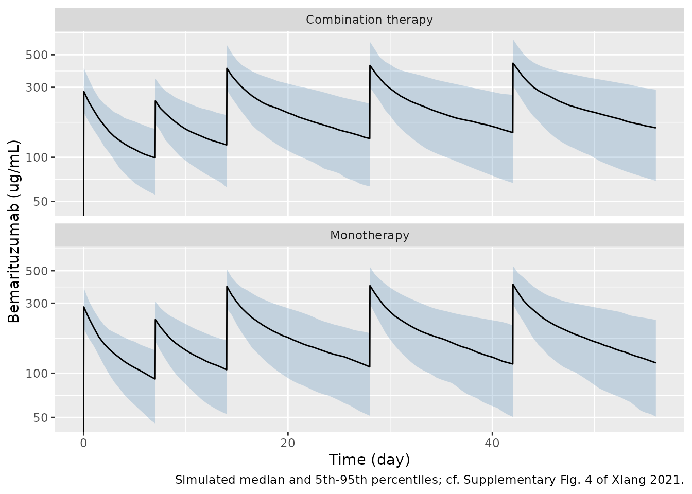
Steady-state exposure by covariate (cf. Figure 2)
Figure 2 of the paper shows the steady-state exposures of the 135 GEA patients (from their individual Bayes estimates) by weight and albumin quartile, sex and therapy. The simulated cohort is shown the same way for sex and therapy.
ss_sim <- sim |>
  dplyr::filter(time >= 350) |>
  dplyr::group_by(id, treatment, SEXF) |>
  dplyr::summarise(
    AUCss = sum(diff(time) * (head(Cc, -1) + tail(Cc, -1)) / 2),
    Cmaxss = max(Cc),
    Ctroughss = Cc[time == 364],
    .groups = "drop"
  )
ss_sim |>
  dplyr::mutate(Sex = ifelse(SEXF == 1, "Female", "Male")) |>
  tidyr::pivot_longer(c(AUCss, Cmaxss, Ctroughss), names_to = "metric") |>
  ggplot(aes(interaction(Sex, treatment, sep = "\n"), value)) +
  geom_boxplot(outlier.size = 0.5) +
  facet_wrap(~metric, scales = "free_y") +
  scale_y_log10() +
  labs(
    x = NULL, y = "Exposure (ug*day/mL or ug/mL)",
    caption = "Simulated steady-state exposures; cf. Figure 2 of Xiang 2021."
  ) +
  theme(axis.text.x = element_text(size = 7))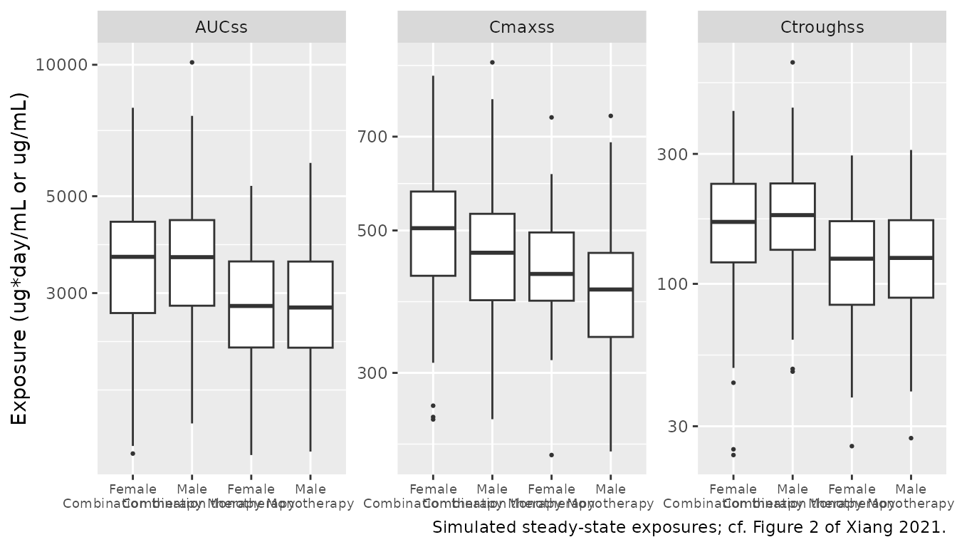
The paper summarises the GEA population (76 patients on combination therapy, 59 on monotherapy) as geometric means of 2805 ug*day/mL (AUCss), 401 ug/mL (Cmax,ss) and 125 ug/mL (Ctrough,ss). The cohort below is weighted to the same therapy mix.
gm_arm <- ss_sim |>
  dplyr::group_by(treatment) |>
  dplyr::summarise(dplyr::across(c(AUCss, Cmaxss, Ctroughss), ~ mean(log(.x))), .groups = "drop")
w <- c("Combination therapy" = 76, "Monotherapy" = 59) / 135
gea_gm <- exp(colSums(as.matrix(gm_arm[, -1]) * w[gm_arm$treatment]))
gea <- data.frame(
  metric = c("AUCss (ug*day/mL)", "Cmax,ss (ug/mL)", "Ctrough,ss (ug/mL)"),
  simulated = gea_gm,
  paper = c(2805, 401, 125)
) |>
  dplyr::mutate(pct_diff = 100 * (simulated / paper - 1))
gea |>
  dplyr::rename(
    "Metric" = metric, "Simulated geometric mean" = simulated,
    "Paper geometric mean" = paper, "Difference (%)" = pct_diff
  ) |>
knitr::kable(digits = 1, row.names = FALSE)| Metric | Simulated geometric mean | Paper geometric mean | Difference (%) |
|---|---|---|---|
| AUCss (ug*day/mL) | 3201.8 | 2805 | 14.1 |
| Cmax,ss (ug/mL) | 442.1 | 401 | 10.3 |
| Ctrough,ss (ug/mL) | 146.0 | 125 | 16.8 |
PKNCA validation
PKNCA on the typical-patient steady-state interval (days 350-364) for the monotherapy and combination-therapy reference patients, compared with the Supplementary Fig. 5 reference values (combination therapy: the reference values times the published +18.8%, +8.6% and +28.6%).
typ_nca <- dplyr::bind_rows(
  typical_ss(ref_cov) |> dplyr::mutate(treatment = "Monotherapy"),
  typical_ss(replace(ref_cov, "CONMED_CHEMO", 1)) |> dplyr::mutate(treatment = "Combination therapy")
) |>
  dplyr::filter(!is.na(Cc)) |>
  dplyr::mutate(id = 1L)
#> ℹ omega/sigma items treated as zero: 'etalcl', 'etalvc', 'etalvp', 'etalvmax'
#> ℹ omega/sigma items treated as zero: 'etalcl', 'etalvc', 'etalvp', 'etalvmax'
typ_conc <- typ_nca |> dplyr::select(id, time, Cc, treatment)
typ_dose <- expand.grid(time = dose_days, treatment = c("Monotherapy", "Combination therapy")) |>
  dplyr::mutate(id = 1L, amt = ifelse(time == 7, 7.5, 15) * 64, duration = 0.5 / 24)

nca_res <- PKNCA::pk.nca(PKNCA::PKNCAdata(
  PKNCA::PKNCAconc(typ_conc, Cc ~ time | treatment + id),
  PKNCA::PKNCAdose(typ_dose, amt ~ time | treatment + id, duration = "duration"),
  intervals = data.frame(start = 350, end = 364, cmax = TRUE, cmin = TRUE, auclast = TRUE)
))

published <- tibble::tribble(
  ~treatment, ~auclast, ~cmax, ~cmin,
  "Monotherapy", 2618.8, 380.3, 113.5,
  "Combination therapy", 2618.8 * 1.188, 380.3 * 1.086, 113.5 * 1.286
)
nlmixr2lib::ncaComparisonTable(
  simulated = nca_res,
  reference = published,
  by = "treatment",
  units = c(auclast = "ug*day/mL", cmax = "ug/mL", cmin = "ug/mL"),
  tolerance_pct = 20
) |>
knitr::kable(caption = "Typical-patient steady-state NCA vs Supplementary Fig. 5. * differs by >20%.")| NCA parameter | treatment | Reference | Simulated | % diff |
|---|---|---|---|---|
| Cmax (ug/mL) | Monotherapy | 380 | 405 | +6.4% |
| Cmax (ug/mL) | Combination therapy | 413 | 449 | +8.7% |
| Cmin (ug/mL) | Monotherapy | 114 | 137 | +21.1%* |
| Cmin (ug/mL) | Combination therapy | 146 | 182 | +24.5%* |
| AUClast (ug*day/mL) | Monotherapy | 2620 | 2960 | +13.2% |
| AUClast (ug*day/mL) | Combination therapy | 3110 | 3620 | +16.3% |
res <- as.data.frame(nca_res$result)
get_par <- function(par, grp) {
  v <- res$PPORRES[res$PPTESTCD == par & res$treatment == grp]
  if (length(v) != 1L) stop("no unique ", par, " for ", grp)
  v
}
auc_mono <- get_par("auclast", "Monotherapy")
# PKNCA agrees with the model's own trapezoid on the same grid, and the
# typical-value offset from the paper is the deterministic one shown above.
stopifnot(
  abs(auc_mono / readings[1, "AUC"] - 1) < 1e-3,
  abs(get_par("cmax", "Monotherapy") / readings[1, "Cmax"] - 1) < 1e-3,
  abs(get_par("cmin", "Monotherapy") / readings[1, "Ctrough"] - 1) < 1e-3
)
AUCss and Cmax,ss are within 20% of the paper’s reference values in both arms; Ctrough,ss is more than 20% above it in both arms (starred), by 21% for monotherapy. The cause is the size of the Michaelis-Menten pathway discussed under “Units of Vmax”.
Assumptions and deviations
- Vmax units. Table 2 labels Vmax as 2.80 ug/day. It is read as 2.80 mg/day, the only reading under which the Michaelis-Menten pathway the paper estimated and retained has any effect, and the one closer to the paper’s own simulations. Even so the typical steady-state exposures run 6-21% above the reference values of Supplementary Fig. 5 and the GEA population means. No clean unit factor on Vmax reconciles all published simulation results; the printed value is kept.
- Sensitivity-analysis bars. The albumin and therapy bars of Supplementary Fig. 5 are about 10-20% smaller than a CL-only covariate can produce with the printed parameters, and the body-weight bars larger. They are reproduced in direction and within 8 percentage points; the covariate ranking differs for AUCss.
- Covariate equation form. Equations 5-8 state the power and exponential forms explicitly; the Results’ percentage statements confirm them.
-
Combination therapy / study. The paper’s indicator
is “combotherapy/ study”, i.e. study FPA144-004 (FIGHT), where every
patient received mFOLFOX6. It is encoded with the canonical
CONMED_CHEMOcolumn. The authors attribute the effect to the first-line population of FIGHT rather than to a drug interaction. - IIV scale. The Results give the final-model CL and Vc variances (0.0854, 0.0221), whose square roots are the Table 2 percentages; the Vp and Vmax percentages are converted the same way, variance = (percent/100)^2.
- No IIV on Q or Km. Table 2 lists IIV on Vmax, CL, Vc and Vp only.
-
Residual error. Equation 4 is an additive error on
log-transformed concentrations with SD 0.146 (Table 2, 14.6%), encoded
as
lnorm(expSd). - Virtual cohort. Weight and albumin distributions are approximations built from the Table 1 medians and ranges; the paper’s individual covariates are not available.