Cemiplimab (Nguyen 2022) • nlmixr2lib

Model and source

Citation: Nguyen J-H, Epling D, Dolphin N, Paccaly A, Conrado D, Davis JD, Al-Huniti N. Population pharmacokinetics modeling and exposure-response analyses of cemiplimab in patients with recurrent or metastatic cervical cancer. CPT Pharmacometrics Syst Pharmacol. 2022;11(11):1458-1471. doi:10.1002/psp4.12855
Description: Two-compartment population PK model for cemiplimab (anti-PD-1 IgG4) with zero-order IV infusion, first-order elimination and a time-varying sigmoid-Emax change in clearance, in adults with solid tumors (CSCC, BCC, NSCLC, other advanced malignancies), updated from the earlier cemiplimab model and externally validated in recurrent or metastatic cervical cancer (Nguyen 2022)
Article: https://doi.org/10.1002/psp4.12855 (open access; Appendix S1 holds the NONMEM control stream of the final model and Tables S1-S11)

Nguyen 2022 updates the earlier cemiplimab population PK model (packaged separately as Yang_2021_cemiplimab) on 1063 patients from four studies: CSCC, BCC, NSCLC and the first-in-human study in advanced malignancies. To stabilise the model the authors removed the IIV on Emax and T50, the covariance between the CL/Q and V1/V2 random effects, and the proportional residual-error component. The updated model was then validated externally on 292 women with recurrent or metastatic cervical cancer (R/M CC) from EMPOWER-Cervical 1, whose data were not used for estimation.

Structure: linear two-compartment model, 30-min IV infusion, with a sigmoid-Emax change in clearance over time since the first dose:

$\mathrm{CL}_i(t) = \mathrm{CL}_{0,i}\, \exp\!\left(\frac{E_{\max,i}\, t^{\gamma}}{T_{50,i}^{\gamma} + t^{\gamma}}\right)$

with $E_{\max} = -0.174$ (CL approaches $e^{-0.174} = 0.840$ of baseline), $T_{50} = 73.7$ days and $\gamma = 2.5$ (fixed). One random effect is shared by CL and Q and one by V1 and V2.

The exposure-response part of the paper (Kaplan-Meier, Cox and logistic regression analyses of OS, PFS, DOR, ORR and irAEs against first-dose exposure) found no exposure-response relationship once baseline albumin, body weight and ECOG status were adjusted for, and reports no parametric exposure-response model, so only the PK model is packaged.

Population

The model-building data set holds 17,312 post-dose concentrations from 1063 patients (Table S2): Study 1423 (first-in-human, advanced malignancies, n = 398), Study 1540 (CSCC, n = 188), Study 1620 (BCC after hedgehog-inhibitor therapy, n = 132) and Study 1624 (PD-L1 >= 50% NSCLC, n = 345). Doses were 1, 3 or 10 mg/kg Q2W, 3 mg/kg Q3W, 200 mg Q2W or 350 mg Q3W, all as 30-min IV infusions (Table S1). Baseline demographics (Table S4): median age 65 years (27-96), median weight 73.2 kg (30.9-171.6), 70.6% male, 87.7% White, median albumin 38.6 g/L (20-93), median ALT 19 IU/L (4-234).

The external-validation cohort (Table S5) was 292 women with R/M CC on 350 mg Q3W: median age 51 years, weight 61.9 kg (35.9-128.7), albumin 39.1 g/L (20-50.7), ALT 14 IU/L (4-101.5), 63.0% White and 29.1% Asian.

The same information is available programmatically via readModelDb("Nguyen_2022_cemiplimab")()$population.

Source trace

Every ini() value carries an in-file comment pointing to its source in inst/modeldb/specificDrugs/Nguyen_2022_cemiplimab.R. Covariate equation forms and reference values come from the Appendix S1 control stream; the final estimates come from Table 1 (the $THETA block of Appendix S1 holds initial estimates only).

Parameter / equation	Value	Source
`lcl` (TVCL0)	log(0.254 L/day)	Table 1
`lq` (TVQ)	log(0.652 L/day)	Table 1
`lvc` (TVV1)	log(3.35 L)	Table 1
`lvp` (TVV2)	log(2.52 L)	Table 1
`cl_time_max` (TVEmax)	-0.174	Table 1
`lcl_t50` (TVT50)	log(73.7 day)	Table 1
`lcl_time_hill` (HILL)	log(2.50), fixed	Table 1, footnote c
`e_wt_cl_q` (CL_WGTBL)	0.539	Table 1
`e_wt_vc_vp` (VssWGTBL)	0.499	Table 1
`e_sexf_cl` (CL_SEX)	-0.137	Table 1
`e_sexf_vc` (V1_SEX)	-0.0801	Table 1
`e_alb_base_vc` (V1_ALBBL)	-0.217	Table 1
`e_alb_cl` (CL_ALB, time-varying)	-1.11	Table 1
`e_alt_cl` (CL_ALTBL)	-0.0729	Table 1
`e_tumtp_cscc_cl` (CL_CSCC)	-0.216	Table 1
`e_tumtp_bcc_cl` (CL_BCC)	-0.211	Table 1
`e_tumtp_bcc_cl_time_max` (Emax_BCC)	-0.872	Table 1
`e_tumtp_other_cl_t50` (T50_OTHER)	-0.491	Table 1
`etalcl` (ETA1, shared CL and Q)	0.0892	Table 1
`etalvc` (ETA2, shared V1 and V2)	0.0709	Table 1
`expSd` (RE)	0.241	Table 1, footnote d
Reference covariates: WT 75 kg, albumin 38.6 g/L, ALT 19 IU/L	–	Appendix S1 `$PK` (`M_WGTBL`, `M_ALBBL`, `M_ALTBL`)
Power covariate forms; `(1 + theta)` forms for sex and tumor type	–	Appendix S1 `$PK`
Q scaled by the CL weight exponent, V2 by the V1 weight exponent	–	Appendix S1 `$PK` (`Q_COV = CLQ_WT`, `V2_COV = Vss_WT`)
Time-dependent CL, `exp(Emax * t^HILL / (T50^HILL + t^HILL))`	–	Table 1 footnote; Appendix S1 `$PK`
Two-compartment ODEs (ADVAN3 TRANS4)	–	Appendix S1
Residual error additive on log concentration, `Y = LOG(CONC) + W*ERR(1)`	–	Appendix S1 `$ERROR`

Virtual cohorts

The observed data are not public. Each study is represented by a virtual cohort of 200 patients whose weight, albumin, ALT and sex follow the per-study medians, ranges and percentages of Table S4 (Table S5 for R/M CC). Weight and ALT are drawn log-normally and albumin normally, each truncated to the published range; the joint covariate structure is not known and is not reproduced. Time-varying albumin is held at its baseline value (ALB = ALB_BASE). Every patient receives 350 mg Q3W for 17 doses (the regimen of Table S7).

set.seed(2022)
n_per <- 200
tau <- 21
n_dose <- 17
dose_times <- seq(0, by = tau, length.out = n_dose)

draw_trunc <- function(n, rfun, lo, hi) pmin(pmax(rfun(n), lo), hi)

# Per-study covariate summaries from Table S4 (Table S5 for R/M CC).
cohort_spec <- tibble::tribble(
  ~cohort,                   ~wt_med, ~wt_lo, ~wt_hi, ~alb_med, ~alb_lo, ~alb_hi, ~alt_med, ~alt_lo, ~alt_hi, ~male_pct, ~cscc, ~bcc, ~other,
  "R/M CC (Study 1676)",       61.9,   35.9,  128.7,     39.1,      20,    50.7,       14,       4,   101.5,         0,     0,    0,      0,
  "CSCC (Study 1540)",         80.7,   31.0,  171.6,     40.0,      25,    48.0,       17,       6,   234.0,      83.0,     1,    0,      0,
  "BCC (Study 1620)",          73.2,   44.6,  134.8,     41.0,      28,    93.0,       16,       5,    69.0,      67.4,     0,    1,      0,
  "NSCLC (Study 1624)",        69.6,   37.6,  138.0,     38.9,      20,    53.5,       17,       4,   133.0,      87.5,     0,    0,      0,
  "All solid tumors (Study 1423)", 75.3, 30.9, 156.0,    37.0,      22,    48.0,       22,       5,   196.0,      51.3,     0,    0,      1
)

make_cohort <- function(spec, id_offset) {
  n <- n_per
  alb <- draw_trunc(n, function(k) rnorm(k, spec$alb_med, 5), spec$alb_lo, spec$alb_hi)
  tibble(
    id = id_offset + seq_len(n),
    cohort = spec$cohort,
    WT = draw_trunc(n, function(k) rlnorm(k, log(spec$wt_med), 0.2), spec$wt_lo, spec$wt_hi),
    ALB_BASE = alb,
    ALB = alb,
    ALT = draw_trunc(n, function(k) rlnorm(k, log(spec$alt_med), 0.5), spec$alt_lo, spec$alt_hi),
    SEXF = rbinom(n, 1, 1 - spec$male_pct / 100),
    TUMTP_CSCC = spec$cscc,
    TUMTP_BCC = spec$bcc,
    TUMTP_OTHER = spec$other
  )
}

subjects <- dplyr::bind_rows(lapply(seq_len(nrow(cohort_spec)), function(i) {
  make_cohort(cohort_spec[i, ], id_offset = (i - 1L) * n_per)
}))
stopifnot(!anyDuplicated(subjects$id))

# Observation grid: dense over the first and the last (steady-state) dosing
# interval, including the end of each 30-min infusion and the trough.
eoi <- 0.5 / 24
ss_start <- dose_times[n_dose]
obs_times <- sort(unique(c(
  0, eoi, seq(1, tau, by = 1),
  seq(tau, ss_start, by = 3),
  ss_start + c(eoi, seq(1, tau, by = 1))
)))

doses <- subjects |>
  tidyr::crossing(time = dose_times) |>
  dplyr::mutate(evid = 1L, amt = 350, dur = eoi, cmt = "central")
obs <- subjects |>
  tidyr::crossing(time = obs_times) |>
  dplyr::mutate(evid = 0L, amt = 0, dur = 0, cmt = "central")
events <- dplyr::bind_rows(doses, obs) |>
  dplyr::arrange(id, time, dplyr::desc(evid)) |>
  dplyr::select(id, time, evid, amt, dur, cmt, dplyr::everything()) |>
  as.data.frame()

Simulation

Table S7 reports population-predicted exposures, i.e. each patient’s typical-value profile at their own covariates with the random effects set to zero. The comparison below therefore uses zeroRe(); a stochastic simulation is used afterwards for the variability-dependent quantities.

mod <- readModelDb("Nguyen_2022_cemiplimab")
mod_typ <- rxode2::zeroRe(mod)
#> ℹ parameter labels from comments will be replaced by 'label()'
sim_typ <- rxode2::rxSolve(
  mod_typ, events = events, keep = "cohort", returnType = "data.frame"
)
#> ℹ omega/sigma items treated as zero: 'etalcl', 'etalvc'
#> Warning: multi-subject simulation without without 'omega'
stopifnot(!anyNA(sim_typ$Cc))

Typical concentration-time profiles by tumor type

sim_typ |>
  dplyr::group_by(cohort, time) |>
  dplyr::summarise(Cc = mean(Cc), .groups = "drop") |>
  ggplot(aes(time, Cc, colour = cohort)) +
  geom_line() +
  labs(
    x = "Time since first dose (day)",
    y = "Cemiplimab concentration (mg/L)",
    colour = NULL,
    title = "Mean population-predicted profiles, 350 mg Q3W",
    caption = "Grid is coarse (every 3 days) between the first and the last dosing interval."
  ) +
  theme_bw() +
  theme(legend.position = "bottom") +
  guides(colour = guide_legend(ncol = 2))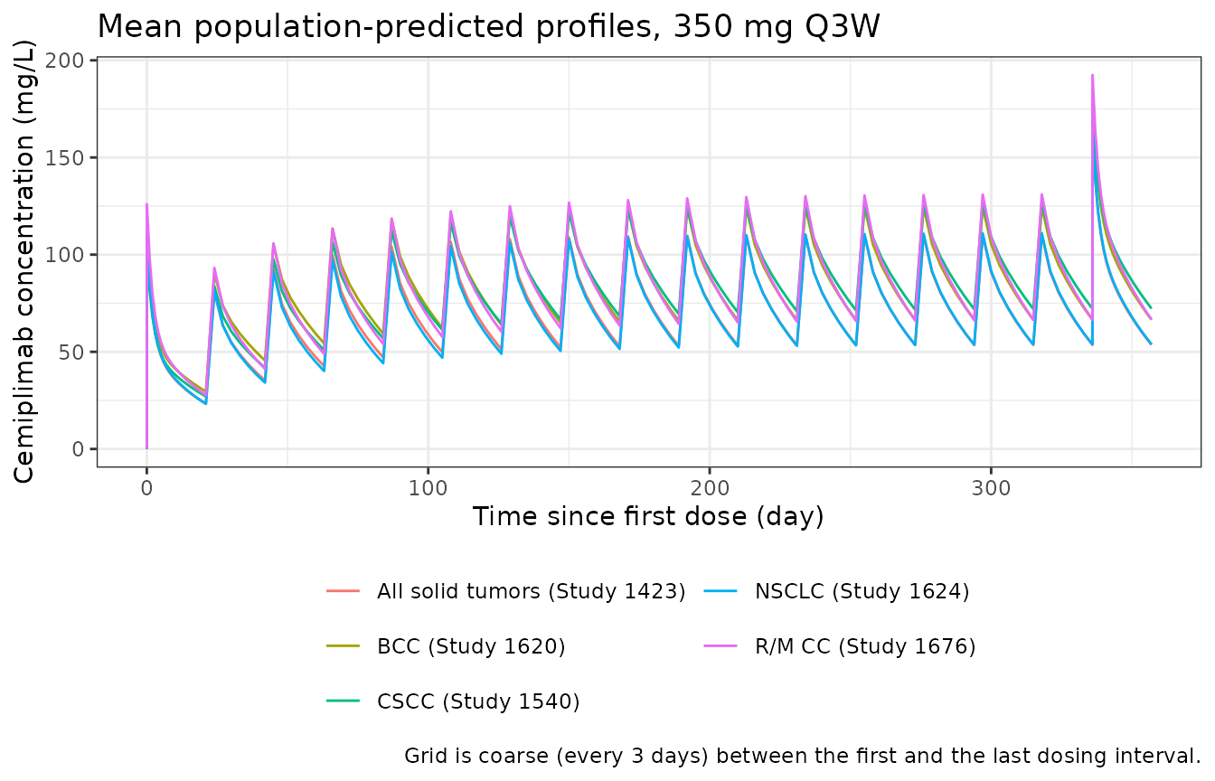

Time-dependent clearance

Typical CL(t) / CL(0) for the reference patient and for the two tumor types that carry an effect on the time course: BCC (Emax reduced by 87.2%) and the other tumor types (T50 reduced by 49.1%).

cl_ratio <- sim_typ |>
  dplyr::filter(cohort %in% c("NSCLC (Study 1624)", "BCC (Study 1620)", "All solid tumors (Study 1423)")) |>
  dplyr::group_by(cohort, time) |>
  dplyr::summarise(ratio = mean(cl / cl_base), .groups = "drop")

ggplot(cl_ratio, aes(time, ratio, colour = cohort)) +
  geom_line() +
  geom_hline(yintercept = exp(-0.174), linetype = "dashed", colour = "grey40") +
  labs(x = "Time since first dose (day)", y = "CL(t) / CL(0)", colour = NULL) +
  theme_bw() +
  theme(legend.position = "bottom")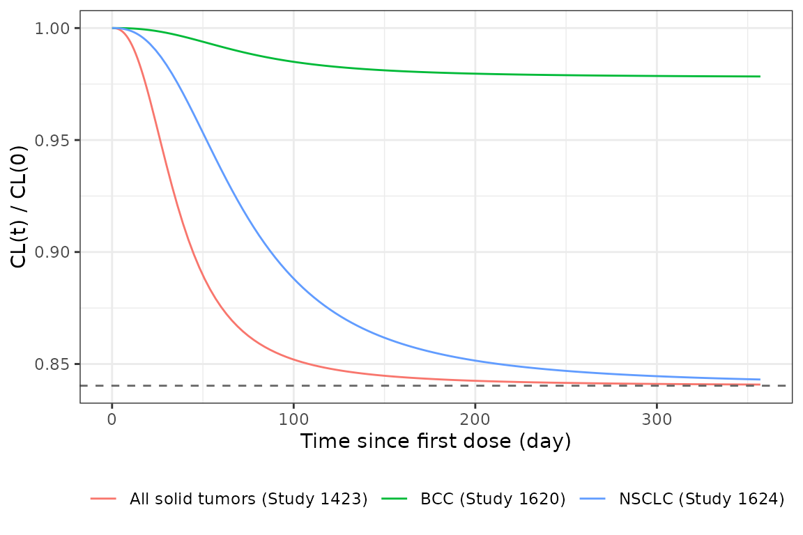


# The asymptote is exp(Emax): 0.840 for the reference and exp(-0.174 *
# 0.128) = 0.978 for BCC. Deterministic (typical values), so the bounds are tight.
ratio_end <- cl_ratio |> dplyr::filter(time == max(time))
stopifnot(
  abs(ratio_end$ratio[ratio_end$cohort == "BCC (Study 1620)"] - exp(-0.174 * 0.128)) < 0.002,
  abs(ratio_end$ratio[ratio_end$cohort == "NSCLC (Study 1624)"] - exp(-0.174)) < 0.01
)

Nguyen 2022 reports a mean 10.8% decrease in CL from the first dose to steady state, generally similar across tumor types except BCC, for which the change was minimal (Table 2: +2.7%). The typical-value curves show the same pattern: about -16% for the reference and other tumor types by the end of the first year, and about -2% for BCC. The post hoc means of Table 2 are smaller because they average over individual albumin trajectories and an unstated steady-state time.

PKNCA: population-predicted exposure (Table S7)

conc <- sim_typ |>
  dplyr::filter(!is.na(Cc)) |>
  dplyr::select(id, time, Cc, cohort)
dose_df <- events |>
  dplyr::filter(evid == 1) |>
  dplyr::select(id, time, amt, cohort)

conc_obj <- PKNCA::PKNCAconc(conc, Cc ~ time | cohort + id, concu = "mg/L", timeu = "day")
dose_obj <- PKNCA::PKNCAdose(dose_df, amt ~ time | cohort + id, doseu = "mg")
intervals <- data.frame(
  start = c(0, ss_start),
  end = c(tau, ss_start + tau),
  cmax = TRUE,
  clast.obs = TRUE,
  auclast = TRUE
)
nca <- PKNCA::pk.nca(PKNCA::PKNCAdata(conc_obj, dose_obj, intervals = intervals))

The trough is the concentration at the end of each 21-day interval (clast.obs); cmin would return the pre-dose zero of the first interval. Table S7 reports means across patients, so the simulated per-patient values are averaged (not pooled by median) before the comparison.

sim_mean <- as.data.frame(nca$result) |>
  dplyr::filter(PPTESTCD %in% c("cmax", "clast.obs", "auclast")) |>
  dplyr::mutate(interval = ifelse(start == 0, "First dose", "Steady state")) |>
  dplyr::group_by(cohort, interval, PPTESTCD) |>
  dplyr::summarise(PPORRES = mean(PPORRES), .groups = "drop")

# Table S7, population-predicted means for 350 mg Q3W.
ref <- tibble::tribble(
  ~cohort,                          ~interval,      ~auclast, ~cmax, ~clast.obs,
  "R/M CC (Study 1676)",            "First dose",        993,   125,  27.3,
  "CSCC (Study 1540)",              "First dose",        949,   113,  27.0,
  "BCC (Study 1620)",               "First dose",        967,   109,  29.3,
  "NSCLC (Study 1624)",             "First dose",        892,   117,  22.8,
  "All solid tumors (Study 1423)",  "First dose",        865,   108,  23.1,
  "R/M CC (Study 1676)",            "Steady state",     1949,   185,  60.1,
  "CSCC (Study 1540)",              "Steady state",     2111,   182,  69.5,
  "BCC (Study 1620)",               "Steady state",     2027,   176,  66.4,
  "NSCLC (Study 1624)",             "Steady state",     1777,   171,  53.8,
  "All solid tumors (Study 1423)",  "Steady state",     1770,   164,  55.2
)

cmp <- nlmixr2lib::ncaComparisonTable(
  simulated = sim_mean,
  reference = ref,
  by = c("cohort", "interval"),
  units = c(cmax = "mg/L", clast.obs = "mg/L", auclast = "day*mg/L")
)
knitr::kable(cmp, caption = "Simulated vs. Table S7 mean population-predicted exposure, 350 mg Q3W (AUC over one 21-day interval; Clast is the trough at day 21 of the interval).")

Simulated vs. Table S7 mean population-predicted exposure, 350 mg Q3W (AUC over one 21-day interval; Clast is the trough at day 21 of the interval).
NCA parameter	cohort	interval	Reference	Simulated	% diff
Cmax (mg/L)	R/M CC (Study 1676)	First dose	125	126	+0.8%
Cmax (mg/L)	R/M CC (Study 1676)	Steady state	185	192	+4.0%
Cmax (mg/L)	CSCC (Study 1540)	First dose	113	103	-9.2%
Cmax (mg/L)	CSCC (Study 1540)	Steady state	182	175	-4.0%
Cmax (mg/L)	BCC (Study 1620)	First dose	109	111	+1.4%
Cmax (mg/L)	BCC (Study 1620)	Steady state	176	177	+0.6%
Cmax (mg/L)	NSCLC (Study 1624)	First dose	117	110	-6.3%
Cmax (mg/L)	NSCLC (Study 1624)	Steady state	171	163	-4.4%
Cmax (mg/L)	All solid tumors (Study 1423)	First dose	108	109	+1.3%
Cmax (mg/L)	All solid tumors (Study 1423)	Steady state	164	163	-0.6%
Clast (mg/L)	R/M CC (Study 1676)	First dose	27.3	27.7	+1.3%
Clast (mg/L)	R/M CC (Study 1676)	Steady state	60.1	66.6	+10.8%
Clast (mg/L)	CSCC (Study 1540)	First dose	27	27.1	+0.2%
Clast (mg/L)	CSCC (Study 1540)	Steady state	69.5	72.3	+4.0%
Clast (mg/L)	BCC (Study 1620)	First dose	29.3	29.5	+0.8%
Clast (mg/L)	BCC (Study 1620)	Steady state	66.4	66.5	+0.2%
Clast (mg/L)	NSCLC (Study 1624)	First dose	22.8	23.3	+2.1%
Clast (mg/L)	NSCLC (Study 1624)	Steady state	53.8	53.9	+0.1%
Clast (mg/L)	All solid tumors (Study 1423)	First dose	23.1	23.2	+0.5%
Clast (mg/L)	All solid tumors (Study 1423)	Steady state	55.2	53.6	-2.9%
AUClast (day*mg/L)	R/M CC (Study 1676)	First dose	993	1010	+1.4%
AUClast (day*mg/L)	R/M CC (Study 1676)	Steady state	1950	2100	+7.9%
AUClast (day*mg/L)	CSCC (Study 1540)	First dose	949	904	-4.7%
AUClast (day*mg/L)	CSCC (Study 1540)	Steady state	2110	2120	+0.6%
AUClast (day*mg/L)	BCC (Study 1620)	First dose	967	976	+1.0%
AUClast (day*mg/L)	BCC (Study 1620)	Steady state	2030	2030	+0.3%
AUClast (day*mg/L)	NSCLC (Study 1624)	First dose	892	876	-1.8%
AUClast (day*mg/L)	NSCLC (Study 1624)	Steady state	1780	1750	-1.4%
AUClast (day*mg/L)	All solid tumors (Study 1423)	First dose	865	868	+0.3%
AUClast (day*mg/L)	All solid tumors (Study 1423)	Steady state	1770	1740	-1.7%

if (!is.null(attr(cmp, "footnote"))) cat(attr(cmp, "footnote"))

pct <- sim_mean |>
  dplyr::inner_join(
    tidyr::pivot_longer(ref, c(auclast, cmax, clast.obs), names_to = "PPTESTCD", values_to = "ref"),
    by = c("cohort", "interval", "PPTESTCD")
  ) |>
  dplyr::mutate(pct_diff = 100 * (PPORRES / ref - 1))
stopifnot(nrow(pct) == 30L)
# The covariate cohorts are random draws from marginal summaries, so assert
# on the centre and a robust envelope (CLAUDE.md, "Vignette assertions over a
# simulated cohort"). A mis-transcribed CL, V1 or unit moves every row by
# tens of percent.
stopifnot(
  abs(median(pct$pct_diff)) < 7,
  quantile(abs(pct$pct_diff), 0.9) < 15
)

The steady-state interval used here is the 17th dose (days 336-357), by which CL has essentially reached its asymptote; the paper does not state which interval its “steady state” refers to. The largest residual gaps are expected for Study 1423, whose patients are represented here entirely as “other tumor types”, whereas the real study also enrolled NSCLC and CSCC patients (it had CSCC expansion cohorts). First-dose exposures agree within about 10% for every cohort, and steady-state exposures within about 5% for the four model-building studies. For R/M CC the simulated steady-state exposures sit roughly 5-11% above Table S7 while the first-dose values match. One possible cause is the time-varying albumin on CL, which is held at baseline here; another is the covariate joint distribution of the real cervical-cancer cohort, which the independent marginal draws do not reproduce.

Post hoc parameters with IIV (Table 2)

A stochastic simulation of the four model-building cohorts reproduces the Table 2 post hoc summaries: CL at first dose, Vss and the first-dose terminal half-life computed from the two-compartment micro-constants.

first <- subjects |>
  dplyr::filter(cohort != "R/M CC (Study 1676)") |>
  dplyr::mutate(time = 0, evid = 0L, amt = 0, dur = 0, cmt = "central") |>
  dplyr::select(id, time, evid, amt, dur, cmt, dplyr::everything()) |>
  as.data.frame()
sim_iiv <- rxode2::rxSolve(mod, events = first, keep = "cohort", returnType = "data.frame")
#> ℹ parameter labels from comments will be replaced by 'label()'
ph <- sim_iiv |>
  dplyr::mutate(
    vss = vc + vp,
    beta = 0.5 * ((kel + k12 + k21) - sqrt((kel + k12 + k21)^2 - 4 * kel * k21)),
    thalf = log(2) / beta
  )
ph_tab <- dplyr::bind_rows(
  ph |> dplyr::mutate(cohort = "All patients"),
  ph
) |>
  dplyr::group_by(cohort) |>
  dplyr::summarise(
    cl_mean = mean(cl), cl_cv = 100 * sd(cl) / mean(cl),
    vss_mean = mean(vss), thalf_mean = mean(thalf),
    .groups = "drop"
  )
ph_ref <- tibble::tribble(
  ~cohort,                          ~cl_ref, ~vss_ref, ~thalf_ref,
  "All patients",                     0.246,     5.89,       19.7,
  "CSCC (Study 1540)",                0.214,     5.86,       21.4,
  "BCC (Study 1620)",                 0.192,     6.07,       24.9,
  "NSCLC (Study 1624)",               0.265,     5.61,       17.5,
  "All solid tumors (Study 1423)",    0.262,     6.10,       19.2
)
ph_cmp <- dplyr::inner_join(ph_ref, ph_tab, by = "cohort")
ph_cmp |>
  dplyr::transmute(
    Cohort = cohort,
    `CL first dose, Table 2 (L/day)` = cl_ref,
    `CL first dose, simulated (L/day)` = signif(cl_mean, 3),
    `CL CV%, simulated` = round(cl_cv, 1),
    `Vss, Table 2 (L)` = vss_ref,
    `Vss, simulated (L)` = signif(vss_mean, 3),
    `t1/2 first dose, Table 2 (day)` = thalf_ref,
    `t1/2 first dose, simulated (day)` = signif(thalf_mean, 3)
  ) |>
  knitr::kable(caption = "Table 2 post hoc means vs. simulated means (random effects included).")

Table 2 post hoc means vs. simulated means (random effects included).
Cohort	CL first dose, Table 2 (L/day)	CL first dose, simulated (L/day)	CL CV%, simulated	Vss, Table 2 (L)	Vss, simulated (L)	t1/2 first dose, Table 2 (day)	t1/2 first dose, simulated (day)
All patients	0.246	0.234	39.6	5.89	6.00	19.7	21.5
CSCC (Study 1540)	0.214	0.216	36.5	5.86	6.28	21.4	24.0
BCC (Study 1620)	0.192	0.199	37.9	6.07	6.05	24.9	25.1
NSCLC (Study 1624)	0.265	0.260	37.8	5.61	5.72	17.5	18.2
All solid tumors (Study 1423)	0.262	0.263	38.0	6.10	5.95	19.2	18.7


ph_pct <- with(ph_cmp, c(
  100 * (cl_mean / cl_ref - 1),
  100 * (vss_mean / vss_ref - 1),
  100 * (thalf_mean / thalf_ref - 1)
))
stopifnot(length(ph_pct) == 15L, abs(median(ph_pct)) < 8, quantile(abs(ph_pct), 0.9) < 20)

The overall CV of CL at first dose in Table 2 is 40.9%; the simulated CV combines the 30.5% CV of the shared CL/Q random effect with the covariate spread of the virtual cohorts.

External validation cohort: R/M CC

Figure 3 of Nguyen 2022 is an external posterior predictive check of the model against 2030 concentrations from 292 R/M CC patients on 350 mg Q3W. The band below is the corresponding model prediction for the virtual R/M CC cohort, with IIV and residual error.

ev_cc <- events |> dplyr::filter(cohort == "R/M CC (Study 1676)", time <= 126)
sim_cc <- rxode2::rxSolve(mod, events = ev_cc, keep = "cohort", returnType = "data.frame")
sim_cc |>
  dplyr::filter(time > 0) |>
  dplyr::group_by(time) |>
  dplyr::summarise(
    med = median(sim), lo = quantile(sim, 0.05), hi = quantile(sim, 0.95),
    .groups = "drop"
  ) |>
  ggplot(aes(time, med)) +
  geom_ribbon(aes(ymin = lo, ymax = hi), alpha = 0.25) +
  geom_line() +
  scale_y_log10() +
  labs(
    x = "Time since first dose (day)",
    y = "Cemiplimab concentration (mg/L)",
    title = "R/M CC, 350 mg Q3W: median and 90% prediction interval",
    caption = "Compare with Figure 3 of Nguyen 2022. N = 200 virtual patients."
  ) +
  theme_bw()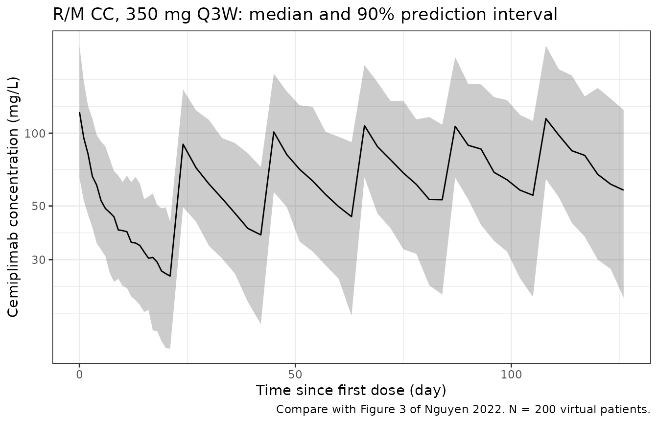

Assumptions and deviations

Final estimates vs. initial estimates. The $THETA block in Appendix S1 lists initial estimates (e.g. TVCL 0.263, TVV2 1.91); the packaged values are the final estimates of Table 1. The control stream supplies the equation forms and the reference covariate values only.
Covariate parameters fixed to zero in the control stream (age, AST, bilirubin, creatinine clearance, serum creatinine, ECOG, ethnicity, race, CSCC and other-tumor effects on Emax, albumin effects on Emax and T50) are absent from Table 1 and are not encoded.
Signed Emax. cl_time_max is negative (CL decreases over time), so it stays on the linear scale; the convention checker’s log-transform warning for this parameter is expected.
Tumor-type coding. The control stream codes CSCC as TUMTYPN = 1, BCC as 2 and “OTHERS” as 5, with no effect for the remaining codes, which include NSCLC. The reference category is therefore NSCLC, and the “other” pool, whose composition the paper does not list, shares the reference CL and Emax but has a shorter T50. The paper does not state which code the R/M CC patients carried in the external validation. The vignette treats them as the reference category; coding them as “other” only shortens T50, which changes steady-state CL by about 4%.
Study 1423 cohort. All virtual Study 1423 patients are coded as “other tumor types”. The real study also enrolled CSCC and NSCLC patients, in proportions the paper does not report.
Albumin. The model uses time-varying albumin on CL and baseline albumin on V1 as separate columns (ALB, ALB_BASE). Albumin trajectories are not reported, so the simulations hold ALB at the baseline value.
Table S7 AUC units. Table S7 labels AUC3wks as mg/L; the values are areas over a 21-day interval and are compared here in day*mg/L.
Weight reference. The control stream normalises weight to 75 kg (M_WGTBL = 75) although the cohort median was 73.2 kg; the packaged model uses 75 kg as published.
Time origin. Time-dependent CL is driven by time since the first dose (ABS(TIME) in the control stream). The packaged model uses rxode2’s t, so the first dose must be given at time 0.
Virtual covariates. Weight, albumin and ALT are drawn independently from marginal distributions anchored at the Table S4 / S5 medians and ranges; their spreads (log-SD 0.2 for weight, SD 5 g/L for albumin, log-SD 0.5 for ALT) were chosen by the maintainers, not reported.