Ritonavir-boosted atazanavir + rifampicin interaction (Kengo 2025)
Source:vignettes/articles/Kengo_2025_atazanavir_ritonavir_rifampicin.Rmd
Kengo_2025_atazanavir_ritonavir_rifampicin.RmdModel and source
- Citation: Kengo A, Resendiz-Galvan JE, Najjemba L, Mugerwa H, De Nicolo A, D’Avolio A, Atoyebi S, Wiesner L, Svensson EM, Waitt C, Denti P (2025). Model-based evaluation of the interaction between ritonavir-boosted atazanavir and rifampicin in Ugandan adults with HIV. Br J Clin Pharmacol 91(12):3471-3481. doi:10.1002/bcp.70195
- Article: https://doi.org/10.1002/bcp.70195
- Supplement (assay methods, Tables S1-S3, Figures S1-S6, and the full
atazanavir NONMEM control stream): supporting information to the same
DOI, distributed by Wiley as
BCP-91-3471-s001.docxand retrievable from Europe PMC as a supplementary file ofPMC12648368.
Ritonavir-boosted atazanavir (ATV/r) is the World Health Organization’s preferred boosted-protease-inhibitor second-line antiretroviral regimen, but rifampicin – the backbone of drug-susceptible tuberculosis treatment – is a strong CYP3A and transporter inducer, and the resulting drug-drug interaction has effectively precluded co-treatment. The DERIVE trial tested whether doubling the ATV/r dosing frequency can overcome that interaction. This paper is the population-pharmacokinetic analysis of DERIVE: it quantifies rifampicin’s effect on atazanavir and ritonavir clearance, bioavailability and absorption, links plasma to intracellular (peripheral blood mononuclear cell, PBMC) concentrations through an effect compartment, and simulates trough target attainment under the three dosing scenarios.
Three of the paper’s four fitted models are packaged here:
mods <- subset(nlmixr2lib::modeldb, grepl("^Kengo_2025", name))[, c("name", "description")]
knitr::kable(
  dplyr::tibble(
    Model = mods$name,
    Role = c(
      "DERIVE atazanavir: plasma + PBMC, ritonavir-boosted, rifampicin regimen covariates",
      "ACTG A5231 atazanavir: plasma only, UNBOOSTED (no ritonavir), rifampicin on F and ka",
      "DERIVE ritonavir: plasma + PBMC, rifampicin regimen covariates"
    )
  )
)| Model | Role |
|---|---|
| Kengo_2025_atazanavir | DERIVE atazanavir: plasma + PBMC, ritonavir-boosted, rifampicin regimen covariates |
| Kengo_2025_atazanavir_a5231 | ACTG A5231 atazanavir: plasma only, UNBOOSTED (no ritonavir), rifampicin on F and ka |
| Kengo_2025_ritonavir | DERIVE ritonavir: plasma + PBMC, rifampicin regimen covariates |
atv <- readModelDb("Kengo_2025_atazanavir")
rtv <- readModelDb("Kengo_2025_ritonavir")
a5231 <- readModelDb("Kengo_2025_atazanavir_a5231")
The paper’s fourth model – the rifampicin one-compartment model with saturable hepatic extraction whose re-estimated parameters are supplementary Table S1 – is deliberately not packaged here. See “Assumptions and deviations” below.
Population
The DERIVE trial (ClinicalTrials.gov NCT04121195) was an open-label, single-arm, dose-escalation study at the Joint Clinical Research Centre in Kampala, Uganda. It enrolled 26 adults living with HIV, virologically suppressed (<50 copies/mL) on ATV/r-based second-line antiretroviral therapy for at least six months, and without tuberculosis or hepatitis co-infection – so rifampicin was given to participants who did not have TB.
Baseline characteristics are Kengo 2025 Table 1: median age 44 years (range 23-61), median weight 67 kg (50-75), median fat-free mass 41.0 kg (37.9-41.9), median height 1.59 m (1.48-1.86), median BMI 26.1 kg/m2 (19.9-31.6), 23 of 26 (88%) female, and all 23 participants with race recorded were Black African. All were on lamivudine; 17 (65%) also on tenofovir disoproxil fumarate, 8 (31%) on zidovudine and 1 (4%) on abacavir.
Sampling ran over four visits with an escalating regimen:
| Visit | Day | Regimen | CONMED_RIF |
REGI_BID |
|---|---|---|---|---|
| 1 | 7 | ATV/r 300/100 mg once daily | 0 | 0 |
| 2 | 21 | + rifampicin 600 mg once daily, + dolutegravir 50 mg twice daily | 1 | 0 |
| 3 | 28 | ATV/r increased to 300/100 mg twice daily | 1 | 1 |
| 4 | 35 | rifampicin increased to 1200 mg once daily | 1 | 1 |
Plasma was drawn predose and at 0.5, 1, 2, 4, 6, 8 and 12 h postdose at every visit, with an extra 24 h sample at visit 1; 857 plasma concentrations entered the analysis (28 atazanavir and 20 ritonavir samples below the limit of quantification). Separate PBMC samples were taken at visits 1, 3 and 4 and at 12 h postdose at visit 2.
The external cohort behind Kengo_2025_atazanavir_a5231
is ACTG A5231 (Kengo 2025 Table S2): 13 healthy adult volunteers in the
United States without HIV, median age 30 years (23-48), median weight 75
kg (55-110), 5 of 13 (38%) female, 1 of 13 (8%) Black, given
unboosted atazanavir 300 mg twice daily alone, then 300
mg twice daily with rifampicin 600 mg once daily, then 400 mg twice
daily with rifampicin, with sampling at the end of each period.
Source trace
Every ini() value in the three model files, with the
source location it came from. Percentages reported as variability are
the omega standard deviation on the log scale, per Kengo 2025 Table 2
footnote c (%CV = sqrt(omega^2) * 100); the model files
store (percentage / 100)^2.
knitr::kable(dplyr::tribble(
  ~Quantity,                                  ~`Kengo_2025_atazanavir`, ~`Kengo_2025_ritonavir`, ~Source,
  "CL/F (L/h) at FFM 42 kg",                  "7.57",   "9.67",   "Table 2",
  "Vc/F (L)",                                 "77.5",   "55.4",   "Table 2",
  "Q/F (L/h)",                                "3.13",   "1.56",   "Table 2",
  "Vp/F (L)",                                 "42.1",   "70.1",   "Table 2",
  "ka (1/h)",                                 "6 fixed", "1.02",  "Table 2",
  "MTT (h)",                                  "0.499",  "0.483",  "Table 2",
  "NN transit compartments",                  "10 fixed", "12.3", "Table 2",
  "F (fraction)",                             "1 fixed", "1 fixed", "Table 2",
  "PBMC equilibration half-life (h)",         "0.963",  "1.40",   "Table 2",
  "PBMC pseudo-partition coefficient",        "0.653",  "1.68",   "Table 2",
  "Fold-change CL, QD + RIF",                 "3.05",   "2.12",   "Table 2",
  "Fold-change CL, BID + RIF",                "2.03",   "same as QD + RIF", "Table 2",
  "Change in F, QD + RIF",                    "-52.5%", "-68.8%", "Table 2",
  "Change in F, BID + RIF",                   "0 (restored)", "-33.3%", "Table 2 / Results 3.4",
  "Change in ka on RIF",                      "-67.3%", "none",   "Table 2",
  "BSV in CL",                                "27.6%",  "16.4%",  "Table 2",
  "BVV in CL",                                "17.5%",  "none",   "Table 2",
  "BOV in ka / MTT / F",                      "97.9% / 59.4% / 48.2%", "82.3% / 43.6% / 55.5%", "Table 2",
  "BOV inflation, unobserved dose",           "1.63",   "none",   "Table 2",
  "Proportional error, plasma",               "19.8%",  "25.6%",  "Table 2",
  "Additive error, plasma (mg/L)",            "0.006 fixed", "0.001 fixed", "Table 2 (= 0.2 x LLOQ)",
  "Proportional error, PBMC",                 "74.9%",  "51.4%",  "Table 2",
  "Additive error, PBMC (mg/L)",              "0.003 fixed", "0.003 fixed", "Table 2 (= 0.2 x LLOQ)",
  "Allometric exponent, CL and Q on FFM",     "0.75 fixed", "0.75 fixed", "Methods 2.3 / control stream",
  "Allometric exponent, Vc and Vp on FFM",    "1 fixed", "1 fixed", "Methods 2.3 / control stream"
))| Quantity | Kengo_2025_atazanavir | Kengo_2025_ritonavir | Source |
|---|---|---|---|
| CL/F (L/h) at FFM 42 kg | 7.57 | 9.67 | Table 2 |
| Vc/F (L) | 77.5 | 55.4 | Table 2 |
| Q/F (L/h) | 3.13 | 1.56 | Table 2 |
| Vp/F (L) | 42.1 | 70.1 | Table 2 |
| ka (1/h) | 6 fixed | 1.02 | Table 2 |
| MTT (h) | 0.499 | 0.483 | Table 2 |
| NN transit compartments | 10 fixed | 12.3 | Table 2 |
| F (fraction) | 1 fixed | 1 fixed | Table 2 |
| PBMC equilibration half-life (h) | 0.963 | 1.40 | Table 2 |
| PBMC pseudo-partition coefficient | 0.653 | 1.68 | Table 2 |
| Fold-change CL, QD + RIF | 3.05 | 2.12 | Table 2 |
| Fold-change CL, BID + RIF | 2.03 | same as QD + RIF | Table 2 |
| Change in F, QD + RIF | -52.5% | -68.8% | Table 2 |
| Change in F, BID + RIF | 0 (restored) | -33.3% | Table 2 / Results 3.4 |
| Change in ka on RIF | -67.3% | none | Table 2 |
| BSV in CL | 27.6% | 16.4% | Table 2 |
| BVV in CL | 17.5% | none | Table 2 |
| BOV in ka / MTT / F | 97.9% / 59.4% / 48.2% | 82.3% / 43.6% / 55.5% | Table 2 |
| BOV inflation, unobserved dose | 1.63 | none | Table 2 |
| Proportional error, plasma | 19.8% | 25.6% | Table 2 |
| Additive error, plasma (mg/L) | 0.006 fixed | 0.001 fixed | Table 2 (= 0.2 x LLOQ) |
| Proportional error, PBMC | 74.9% | 51.4% | Table 2 |
| Additive error, PBMC (mg/L) | 0.003 fixed | 0.003 fixed | Table 2 (= 0.2 x LLOQ) |
| Allometric exponent, CL and Q on FFM | 0.75 fixed | 0.75 fixed | Methods 2.3 / control stream |
| Allometric exponent, Vc and Vp on FFM | 1 fixed | 1 fixed | Methods 2.3 / control stream |
The Kengo_2025_atazanavir_a5231 file traces to
supplementary Table S3, whose own note reads “All fixed parameters are
estimates from DERIVE study population”: CL 7.55 L/h, Vc 77.3 L, Q 3.51
L/h, Vp 48.9 L, ka 6 1/h, NN 10, F 1, the -70.8% rifampicin effect on
ka, and the 18.8% / 0.005 mg/L residual error are all carried over
fixed, while the 2.13-fold clearance increase in the absence of
ritonavir, the -55.3% rifampicin effect on bioavailability, the 1.38 h
mean transit time, the 18.8% between-subject variability in clearance,
the 48.1% and 58.3% between-occasion variabilities and the 1.7-fold
unobserved-dose inflation were estimated on the A5231 data.
The structure of all three files – the Savic analytical transit chain
feeding a first-order depot, the two-compartment disposition, the
fat-free-mass allometry, and the PBMC state that integrates a
concentration
(d/dt(effect) = ke0 * (ppc * Cc - effect)) – is taken
verbatim from the atazanavir NONMEM control stream printed in the
supplement, whose $DES reads
DADT(1) = TRANSIT - KA*A(1)
DADT(2) = KA*A(1) - K*A(2) + K32*A(3) - K23*A(2)
DADT(3) = K23*A(2) - K32*A(3)
DADT(4) = KE0*(PPC*C2 - A(4))
with C2 = A(2)/V and TRANSIT the Savic
gamma-density closed form that rxode2::transit()
implements.
Virtual cohort
The cohort reproduces the DERIVE demographics of Table 1 and derives
fat-free mass with the Janmahasatian formula the control stream uses, so
the derivation documented in each model’s
covariateData[[FFM]]$notes is exercised rather than
assumed. Two hundred participants per arm – the library cap – is ample
for the trough distributions below.
set.seed(20251114)

n_per_arm <- 200

janmahasatian_ffm <- function(wt, ht_m, sexf) {
  whsmax <- ifelse(sexf == 1, 37.99, 42.92)
  whs50 <- ifelse(sexf == 1, 35.98, 30.93)
  ht2 <- ht_m^2
  whsmax * ht2 * wt / (whs50 * ht2 + wt)
}

rtrunc <- function(n, mean, sd, lo, hi) {
  x <- stats::rnorm(n, mean, sd)
  pmin(pmax(x, lo), hi)
}

subjects <- dplyr::tibble(
  subject = seq_len(n_per_arm),
  SEXF = stats::rbinom(n_per_arm, 1L, 0.88),
  WT = rtrunc(n_per_arm, 66, 7, 50, 75)
) |>
  dplyr::mutate(
    HT = ifelse(SEXF == 1,
                rtrunc(dplyr::n(), 1.585, 0.060, 1.48, 1.86),
                rtrunc(dplyr::n(), 1.700, 0.070, 1.48, 1.86)),
    FFM = janmahasatian_ffm(WT, HT, SEXF)
  )

knitr::kable(
  dplyr::tibble(
    Characteristic = c("Female (%)", "Weight (kg)", "Height (m)", "Fat-free mass (kg)"),
    `Virtual cohort, median (range)` = c(
      sprintf("%.0f", 100 * mean(subjects$SEXF)),
      sprintf("%.1f (%.1f-%.1f)", median(subjects$WT), min(subjects$WT), max(subjects$WT)),
      sprintf("%.2f (%.2f-%.2f)", median(subjects$HT), min(subjects$HT), max(subjects$HT)),
      sprintf("%.1f (%.1f-%.1f)", median(subjects$FFM), min(subjects$FFM), max(subjects$FFM))
    ),
    `Kengo 2025 Table 1` = c("88", "67 (50-75)", "1.59 (1.48-1.86)", "41.0 (37.9-41.9)")
  ),
  caption = "Virtual cohort against the DERIVE baseline characteristics."
)| Characteristic | Virtual cohort, median (range) | Kengo 2025 Table 1 |
|---|---|---|
| Female (%) | 88 | 88 |
| Weight (kg) | 64.4 (50.0-75.0) | 67 (50-75) |
| Height (m) | 1.60 (1.48-1.80) | 1.59 (1.48-1.86) |
| Fat-free mass (kg) | 40.1 (32.3-58.8) | 41.0 (37.9-41.9) |
# The derived fat-free mass must land on the cohort value the model is
# referenced to. Assert on the centre, not on the extremes: the tails of a
# random cohort are not reproducible across rxode2 builds.
stopifnot(abs(median(subjects$FFM) - 41.0) < 2.5)
The derived median fat-free mass reproduces Table 1’s 41.0 kg, which is the check that matters: it confirms the Janmahasatian formula, the sex coding and the height distribution together give the size descriptor the model expects. The cohort’s fat-free-mass spread is wider than the 37.9-41.9 kg Table 1 prints, which is discussed in the Errata.
Simulation
Every arm is dosed over the same 720 h (30 day) horizon and observed over its final dosing interval. That horizon is set by the slowest drug in the pair: with the Table 2 estimates, ritonavir’s terminal half-life is about 37 h without rifampicin, so the eight dosing occasions the model carries would leave the twice-daily arm only ~2.6 half-lives in and well short of steady state. Thirty QD or sixty BID doses put every arm past ten half-lives.
The occasion index therefore cycles,
OCC = ((dose index - 1) mod 8) + 1, so each dose still
draws a between-occasion effect of the right magnitude from the eight
etas the source control stream’s
IF (OCC==1) ... IF (OCC==8) multiplexers define; doses
beyond the eighth reuse an earlier occasion’s draw. Because all eight
occasions share one variance this preserves the distribution of the
trough, which is what the target-attainment comparison depends on.
SELFADMIN is 0 throughout: these are directly observed
doses, so the 1.63-fold inflation of the absorption random effects does
not apply.
t_end <- 720  # h; >= 10 terminal half-lives for both drugs in every arm
n_occ <- 8    # occasions the models carry

make_arm <- function(dose, ii, rif, bid, label, id_offset, by = 0.25) {
  n_dose <- t_end / ii
  ids <- id_offset + subjects$subject
  cov <- subjects |>
    dplyr::mutate(id = ids) |>
    dplyr::select(id, FFM, WT, SEXF)

  dosing <- tidyr::expand_grid(id = ids, time = seq(0, ii * (n_dose - 1), by = ii)) |>
    dplyr::mutate(amt = dose, evid = 1L, cmt = "depot", dvid = NA_integer_)
  # The DERIVE models declare two endpoints (Cc and Cpbmc), so every
  # observation row has to nominate one. The right way to do that is the
  # `dvid` column, never the endpoint name in the compartment column: naming an
  # algebraic observable as a compartment makes rxode2 inject a slot for it and
  # renumber the
  # ODE states, which is the documented slot-renumbering trap. Observations are
  # therefore written on the ODE state `central`, with dvid = 1 selecting the
  # plasma endpoint; rxSolve returns both Cc and Cpbmc as columns regardless.
  obs <- tidyr::expand_grid(id = ids, time = seq(ii * (n_dose - 1), t_end, by = by)) |>
    dplyr::mutate(amt = NA_real_, evid = 0L, cmt = "central", dvid = 1L)

  dplyr::bind_rows(dosing, obs) |>
    dplyr::left_join(cov, by = "id") |>
    dplyr::mutate(
      CONMED_RIF = rif,
      REGI_BID = bid,
      SELFADMIN = 0,
      OCC = as.integer(floor(time / ii)) %% n_occ + 1L,
      treatment = label,
      tau = ii,
      last_dose_time = ii * (n_dose - 1)
    ) |>
    dplyr::arrange(id, time, dplyr::desc(evid))
}

arms <- dplyr::bind_rows(
  make_arm(300, 24, 0, 0, "ATV/r QD",           0L),
  make_arm(300, 24, 1, 0, "ATV/r QD + RIF",  1000L),
  make_arm(300, 12, 1, 1, "ATV/r BID + RIF", 2000L)
)
stopifnot(!anyDuplicated(arms[, c("id", "time", "evid")]))
set.seed(20251114)
sim_atv <- rxode2::rxSolve(
  atv, events = arms,
  keep = c("treatment", "FFM", "WT", "SEXF", "tau", "last_dose_time"),
  useLinCmt = FALSE
) |>
  as.data.frame() |>
  dplyr::filter(!is.na(Cc))
#> ℹ parameter labels from comments will be replaced by 'label()'
#> Warning: some etas defaulted to non-mu referenced, possible parsing error: etabvv_cl_1, etabvv_cl_2, etabvv_cl_3, etabvv_cl_4, etaiov_ka_1, etaiov_ka_2, etaiov_ka_3, etaiov_ka_4, etaiov_ka_5, etaiov_ka_6, etaiov_ka_7, etaiov_ka_8, etaiov_mtt_1, etaiov_mtt_2, etaiov_mtt_3, etaiov_mtt_4, etaiov_mtt_5, etaiov_mtt_6, etaiov_mtt_7, etaiov_mtt_8, etaiov_fdepot_1, etaiov_fdepot_2, etaiov_fdepot_3, etaiov_fdepot_4, etaiov_fdepot_5, etaiov_fdepot_6, etaiov_fdepot_7, etaiov_fdepot_8
#> as a work-around try putting the mu-referenced expression on a simple line

set.seed(20251114)  # common random numbers across the two drugs
sim_rtv <- rxode2::rxSolve(
  rtv, events = dplyr::mutate(arms, amt = ifelse(evid == 1L, 100, amt)),
  keep = c("treatment", "FFM", "WT", "SEXF", "tau", "last_dose_time"),
  useLinCmt = FALSE
) |>
  as.data.frame() |>
  dplyr::filter(!is.na(Cc))
#> ℹ parameter labels from comments will be replaced by 'label()'
#> Warning: some etas defaulted to non-mu referenced, possible parsing error: etaiov_ka_1, etaiov_ka_2, etaiov_ka_3, etaiov_ka_4, etaiov_ka_5, etaiov_ka_6, etaiov_ka_7, etaiov_ka_8, etaiov_mtt_1, etaiov_mtt_2, etaiov_mtt_3, etaiov_mtt_4, etaiov_mtt_5, etaiov_mtt_6, etaiov_mtt_7, etaiov_mtt_8, etaiov_fdepot_1, etaiov_fdepot_2, etaiov_fdepot_3, etaiov_fdepot_4, etaiov_fdepot_5, etaiov_fdepot_6, etaiov_fdepot_7, etaiov_fdepot_8
#> as a work-around try putting the mu-referenced expression on a simple line

stopifnot(
  dplyr::n_distinct(sim_atv$id) == 3 * n_per_arm,
  dplyr::n_distinct(sim_rtv$id) == 3 * n_per_arm,
  all(is.finite(sim_atv$Cc)), all(is.finite(sim_atv$Cpbmc)),
  all(is.finite(sim_rtv$Cc)), all(is.finite(sim_rtv$Cpbmc))
)
The typical-value profiles use rxode2::zeroRe() on one
representative participant per arm, held at the model’s own reference
size of 42 kg fat-free mass so the curves are the published typical
values with no cohort assumption.
# A finer observation grid than the cohort arms: the structural identities
# below integrate and re-integrate these profiles, and atazanavir's fixed
# ka of 6 1/h makes the absorption peak sharp enough that a 0.25 h grid would
# limit the trapezoidal and interpolation accuracy. Only three participants
# are solved here, so the finer grid is cheap.
typical_arms <- dplyr::bind_rows(
  make_arm(300, 24, 0, 0, "ATV/r QD",           0L, by = 0.02),
  make_arm(300, 24, 1, 0, "ATV/r QD + RIF",  1000L, by = 0.02),
  make_arm(300, 12, 1, 1, "ATV/r BID + RIF", 2000L, by = 0.02)
) |>
  dplyr::filter(id %in% c(1L, 1001L, 2001L)) |>
  dplyr::mutate(FFM = 42)

sim_atv_typ <- rxode2::rxSolve(
  rxode2::zeroRe(atv), events = typical_arms,
  keep = c("treatment", "tau", "last_dose_time"), useLinCmt = FALSE
) |>
  as.data.frame() |>
  dplyr::filter(!is.na(Cc))
#> ℹ parameter labels from comments will be replaced by 'label()'
#> Warning: some etas defaulted to non-mu referenced, possible parsing error: etabvv_cl_1, etabvv_cl_2, etabvv_cl_3, etabvv_cl_4, etaiov_ka_1, etaiov_ka_2, etaiov_ka_3, etaiov_ka_4, etaiov_ka_5, etaiov_ka_6, etaiov_ka_7, etaiov_ka_8, etaiov_mtt_1, etaiov_mtt_2, etaiov_mtt_3, etaiov_mtt_4, etaiov_mtt_5, etaiov_mtt_6, etaiov_mtt_7, etaiov_mtt_8, etaiov_fdepot_1, etaiov_fdepot_2, etaiov_fdepot_3, etaiov_fdepot_4, etaiov_fdepot_5, etaiov_fdepot_6, etaiov_fdepot_7, etaiov_fdepot_8
#> as a work-around try putting the mu-referenced expression on a simple line
#> Warning: some etas defaulted to non-mu referenced, possible parsing error: etabvv_cl_1, etabvv_cl_2, etabvv_cl_3, etabvv_cl_4, etaiov_ka_1, etaiov_ka_2, etaiov_ka_3, etaiov_ka_4, etaiov_ka_5, etaiov_ka_6, etaiov_ka_7, etaiov_ka_8, etaiov_mtt_1, etaiov_mtt_2, etaiov_mtt_3, etaiov_mtt_4, etaiov_mtt_5, etaiov_mtt_6, etaiov_mtt_7, etaiov_mtt_8, etaiov_fdepot_1, etaiov_fdepot_2, etaiov_fdepot_3, etaiov_fdepot_4, etaiov_fdepot_5, etaiov_fdepot_6, etaiov_fdepot_7, etaiov_fdepot_8
#> as a work-around try putting the mu-referenced expression on a simple line
#> ℹ omega/sigma items treated as zero: 'etalcl', 'etabvv_cl_1', 'etabvv_cl_2', 'etabvv_cl_3', 'etabvv_cl_4', 'etaiov_ka_1', 'etaiov_ka_2', 'etaiov_ka_3', 'etaiov_ka_4', 'etaiov_ka_5', 'etaiov_ka_6', 'etaiov_ka_7', 'etaiov_ka_8', 'etaiov_mtt_1', 'etaiov_mtt_2', 'etaiov_mtt_3', 'etaiov_mtt_4', 'etaiov_mtt_5', 'etaiov_mtt_6', 'etaiov_mtt_7', 'etaiov_mtt_8', 'etaiov_fdepot_1', 'etaiov_fdepot_2', 'etaiov_fdepot_3', 'etaiov_fdepot_4', 'etaiov_fdepot_5', 'etaiov_fdepot_6', 'etaiov_fdepot_7', 'etaiov_fdepot_8'
#> Warning: multi-subject simulation without without 'omega'

sim_rtv_typ <- rxode2::rxSolve(
  rxode2::zeroRe(rtv),
  events = dplyr::mutate(typical_arms, amt = ifelse(evid == 1L, 100, amt)),
  keep = c("treatment", "tau", "last_dose_time"), useLinCmt = FALSE
) |>
  as.data.frame() |>
  dplyr::filter(!is.na(Cc))
#> ℹ parameter labels from comments will be replaced by 'label()'
#> Warning: some etas defaulted to non-mu referenced, possible parsing error: etaiov_ka_1, etaiov_ka_2, etaiov_ka_3, etaiov_ka_4, etaiov_ka_5, etaiov_ka_6, etaiov_ka_7, etaiov_ka_8, etaiov_mtt_1, etaiov_mtt_2, etaiov_mtt_3, etaiov_mtt_4, etaiov_mtt_5, etaiov_mtt_6, etaiov_mtt_7, etaiov_mtt_8, etaiov_fdepot_1, etaiov_fdepot_2, etaiov_fdepot_3, etaiov_fdepot_4, etaiov_fdepot_5, etaiov_fdepot_6, etaiov_fdepot_7, etaiov_fdepot_8
#> as a work-around try putting the mu-referenced expression on a simple line
#> Warning: some etas defaulted to non-mu referenced, possible parsing error: etaiov_ka_1, etaiov_ka_2, etaiov_ka_3, etaiov_ka_4, etaiov_ka_5, etaiov_ka_6, etaiov_ka_7, etaiov_ka_8, etaiov_mtt_1, etaiov_mtt_2, etaiov_mtt_3, etaiov_mtt_4, etaiov_mtt_5, etaiov_mtt_6, etaiov_mtt_7, etaiov_mtt_8, etaiov_fdepot_1, etaiov_fdepot_2, etaiov_fdepot_3, etaiov_fdepot_4, etaiov_fdepot_5, etaiov_fdepot_6, etaiov_fdepot_7, etaiov_fdepot_8
#> as a work-around try putting the mu-referenced expression on a simple line
#> ℹ omega/sigma items treated as zero: 'etalcl', 'etaiov_ka_1', 'etaiov_ka_2', 'etaiov_ka_3', 'etaiov_ka_4', 'etaiov_ka_5', 'etaiov_ka_6', 'etaiov_ka_7', 'etaiov_ka_8', 'etaiov_mtt_1', 'etaiov_mtt_2', 'etaiov_mtt_3', 'etaiov_mtt_4', 'etaiov_mtt_5', 'etaiov_mtt_6', 'etaiov_mtt_7', 'etaiov_mtt_8', 'etaiov_fdepot_1', 'etaiov_fdepot_2', 'etaiov_fdepot_3', 'etaiov_fdepot_4', 'etaiov_fdepot_5', 'etaiov_fdepot_6', 'etaiov_fdepot_7', 'etaiov_fdepot_8'
#> Warning: multi-subject simulation without without 'omega'
Structural checks against printed values
These are closed-form identities of the encoded model, evaluated on the solved profiles and compared against numbers printed in Kengo 2025. Because the two sides are compared at typical values with the random effects zeroed, the only difference is ODE-solver error, so the tolerances are tight.
The PBMC effect compartment equilibrates to the printed pseudo-partition coefficient
For a Sheiner effect compartment
d Ce / dt = ke0 * (ppc * Cc - Ce), integrating over one
complete steady-state dosing interval gives
Ce(tau) - Ce(0) = 0 = ke0 * (ppc * INT(Cc) - INT(Ce)),
hence INT(Ce) / INT(Cc) = ppc exactly, whatever the shape
of Cc(t) and whatever ke0 is. The ratio
therefore recovers the printed pseudo-partition coefficient and is
independent of the equilibration half-life.
trap <- function(t, y) sum(diff(t) * (utils::head(y, -1) + utils::tail(y, -1)) / 2)

ppc_check <- dplyr::bind_rows(
  sim_atv_typ |> dplyr::mutate(drug = "Atazanavir"),
  sim_rtv_typ |> dplyr::mutate(drug = "Ritonavir")
) |>
  dplyr::group_by(drug, treatment) |>
  dplyr::summarise(ppc_simulated = trap(time, Cpbmc) / trap(time, Cc), .groups = "drop") |>
  dplyr::mutate(ppc_published = ifelse(drug == "Atazanavir", 0.653, 1.68))

knitr::kable(
  ppc_check |>
    dplyr::mutate(`% diff` = 100 * (ppc_simulated - ppc_published) / ppc_published) |>
    dplyr::rename("Drug" = drug, "Scenario" = treatment,
                  "PPC simulated" = ppc_simulated, "PPC published (Table 2)" = ppc_published),
  digits = 4,
  caption = "Steady-state PBMC-to-plasma exposure ratio against the published pseudo-partition coefficient."
)| Drug | Scenario | PPC simulated | PPC published (Table 2) | % diff |
|---|---|---|---|---|
| Atazanavir | ATV/r BID + RIF | 0.653 | 0.653 | 0 |
| Atazanavir | ATV/r QD | 0.653 | 0.653 | 0 |
| Atazanavir | ATV/r QD + RIF | 0.653 | 0.653 | 0 |
| Ritonavir | ATV/r BID + RIF | 1.680 | 1.680 | 0 |
| Ritonavir | ATV/r QD | 1.680 | 1.680 | 0 |
| Ritonavir | ATV/r QD + RIF | 1.680 | 1.680 | 0 |
The ratio reproduces 0.653 for atazanavir and 1.68 for ritonavir in every scenario, which is also the paper’s finding that neither PBMC parameter was affected by rifampicin (Results 3.5). Ritonavir’s coefficient above 1 means it concentrates in PBMCs relative to plasma, whereas atazanavir does not.
The equilibration half-life reproduces on an independent re-integration
ppc sets the level the effect compartment reaches;
ke0 sets how fast. The check below re-integrates
d Ce / dt = ke0 * (ppc * Cc - Ce) outside rxode2, driving
it with the solved plasma profile and the published equilibration
half-lives (0.963 h atazanavir, 1.40 h ritonavir), and compares against
the model’s own Cpbmc.
# Exact step solution of d Ce / dt = ke0 * (ppc * Cc - Ce) when the driver Cc
# is linear across the step, Cc(s) = a + b*s:
#   Ce(dt) = ppc*(a + b*dt - b/ke0) + (Ce0 - ppc*(a - b/ke0)) * exp(-ke0*dt)
# The initial condition is taken from the model's own first Cpbmc value,
# because what is under test is the equilibration DYNAMICS, not where the
# steady-state interval happens to start.
reintegrate_effect <- function(time, cc, ce0, thalf, ppc) {
  ke0 <- log(2) / thalf
  ce <- numeric(length(time))
  ce[1] <- ce0
  for (i in seq_along(time)[-1]) {
    dt <- time[i] - time[i - 1]
    a <- cc[i - 1]
    b <- (cc[i] - cc[i - 1]) / dt
    ce[i] <- ppc * (a + b * dt - b / ke0) +
      (ce[i - 1] - ppc * (a - b / ke0)) * exp(-ke0 * dt)
  }
  ce
}

ke0_check <- dplyr::bind_rows(
  sim_atv_typ |> dplyr::mutate(drug = "Atazanavir", thalf = 0.963, ppc = 0.653),
  sim_rtv_typ |> dplyr::mutate(drug = "Ritonavir", thalf = 1.40, ppc = 1.68)
) |>
  dplyr::group_by(drug, treatment) |>
  dplyr::arrange(time, .by_group = TRUE) |>
  dplyr::mutate(
    Cpbmc_reintegrated = reintegrate_effect(time, Cc, Cpbmc[1], thalf[1], ppc[1])
  ) |>
  dplyr::summarise(
    max_rel_diff = max(abs(Cpbmc_reintegrated - Cpbmc)) / max(Cpbmc),
    .groups = "drop"
  )

knitr::kable(
  ke0_check |>
    dplyr::rename("Drug" = drug, "Scenario" = treatment,
                  "Max |difference| / max(Cpbmc)" = max_rel_diff),
  digits = 5,
  caption = "Model Cpbmc against an independent re-integration using the published equilibration half-life."
)| Drug | Scenario | Max |difference| / max(Cpbmc) |
|---|---|---|
| Atazanavir | ATV/r BID + RIF | 3e-05 |
| Atazanavir | ATV/r QD | 5e-05 |
| Atazanavir | ATV/r QD + RIF | 4e-05 |
| Ritonavir | ATV/r BID + RIF | 3e-05 |
| Ritonavir | ATV/r QD | 2e-05 |
| Ritonavir | ATV/r QD + RIF | 3e-05 |
The regimen covariates reproduce the printed fold-changes
At steady state and at typical values,
AUC(0-tau) = F * Dose / CL, so the ratio of daily exposures
between two arms is the ratio of their bioavailability factors divided
by the ratio of their clearance factors. Every expected value below is
computed from numbers printed in Kengo 2025 Table 2, not from the model
object.
daily_auc <- function(sim) {
  sim |>
    dplyr::group_by(treatment) |>
    dplyr::summarise(auc_tau = trap(time, Cc), tau = tau[1], .groups = "drop") |>
    dplyr::mutate(auc_daily = auc_tau * 24 / tau)
}

# `expected` is a NAMED vector keyed by treatment and joined by name, never
# positionally: dplyr::summarise() returns groups in alphabetical order, which
# is not the order the scenarios are written in.
ratio_table <- function(sim, drug, expected) {
  d <- daily_auc(sim)
  ref <- d$auc_daily[d$treatment == "ATV/r QD"]
  stopifnot(length(ref) == 1L, all(d$treatment %in% names(expected)))
  dplyr::tibble(
    Drug = drug,
    Scenario = d$treatment,
    `Daily AUC ratio vs ATV/r QD, simulated` = d$auc_daily / ref,
    `Expected from Table 2` = unname(expected[d$treatment])
  )
}

# Atazanavir: QD + RIF     -> F 0.475, CL x3.05  -> 0.475 / 3.05
#             BID + RIF    -> F restored to 1, CL x2.03, double daily dose -> 2 / 2.03
# Ritonavir:  QD + RIF     -> F 0.312, CL x2.12  -> 0.312 / 2.12
#             BID + RIF    -> F 0.667, CL x2.12, double daily dose -> 2 * 0.667 / 2.12
regimen_check <- dplyr::bind_rows(
  ratio_table(sim_atv_typ, "Atazanavir", c(
    "ATV/r QD" = 1,
    "ATV/r QD + RIF" = (1 - 0.525) / 3.05,
    "ATV/r BID + RIF" = 2 / 2.03
  )),
  ratio_table(sim_rtv_typ, "Ritonavir", c(
    "ATV/r QD" = 1,
    "ATV/r QD + RIF" = (1 - 0.688) / 2.12,
    "ATV/r BID + RIF" = 2 * (1 - 0.333) / 2.12
  ))
) |>
  dplyr::mutate(`% diff` = 100 * (`Daily AUC ratio vs ATV/r QD, simulated` /
                                    `Expected from Table 2` - 1))

knitr::kable(regimen_check, digits = 4,
caption = "Simulated steady-state daily exposure ratios against the Table 2 fold-changes.")| Drug | Scenario | Daily AUC ratio vs ATV/r QD, simulated | Expected from Table 2 | % diff |
|---|---|---|---|---|
| Atazanavir | ATV/r BID + RIF | 0.9852 | 0.9852 | 0 |
| Atazanavir | ATV/r QD | 1.0000 | 1.0000 | 0 |
| Atazanavir | ATV/r QD + RIF | 0.1557 | 0.1557 | 0 |
| Ritonavir | ATV/r BID + RIF | 0.6292 | 0.6292 | 0 |
| Ritonavir | ATV/r QD | 1.0000 | 1.0000 | 0 |
| Ritonavir | ATV/r QD + RIF | 0.1472 | 0.1472 | 0 |
This reproduces the paper’s central result. For atazanavir the daily
exposure ratio under twice-daily ATV/r with rifampicin is
2 / 2.03 = 0.985: doubling the dosing frequency very nearly
restores daily exposure, because the bioavailability loss is abolished
and the residual clearance induction is exactly offset by the doubled
daily dose. For ritonavir the same manoeuvre only reaches
0.629, i.e. exposure is partially restored – which
is Results 3.4 verbatim.
Allometric scaling
Clearance scales as (FFM / 42)^0.75 and volumes as
(FFM / 42)^1, so daily exposure at typical values must
scale as (FFM / 42)^-0.75.
allo_grid <- typical_arms |>
  dplyr::filter(treatment == "ATV/r QD") |>
  tidyr::expand_grid(ffm_test = c(35, 42, 55)) |>
  dplyr::mutate(FFM = ffm_test, id = as.integer(id + 10 * ffm_test)) |>
  dplyr::arrange(id, time, dplyr::desc(evid))

allo <- rxode2::rxSolve(rxode2::zeroRe(atv), events = allo_grid,
                        keep = c("treatment", "ffm_test"), useLinCmt = FALSE) |>
  as.data.frame() |>
  dplyr::filter(!is.na(Cc)) |>
  dplyr::group_by(ffm_test) |>
  dplyr::summarise(auc = trap(time, Cc), .groups = "drop") |>
  dplyr::mutate(
    ratio_simulated = auc / auc[ffm_test == 42],
    ratio_expected = (ffm_test / 42)^-0.75
  )
#> ℹ parameter labels from comments will be replaced by 'label()'
#> Warning: some etas defaulted to non-mu referenced, possible parsing error: etabvv_cl_1, etabvv_cl_2, etabvv_cl_3, etabvv_cl_4, etaiov_ka_1, etaiov_ka_2, etaiov_ka_3, etaiov_ka_4, etaiov_ka_5, etaiov_ka_6, etaiov_ka_7, etaiov_ka_8, etaiov_mtt_1, etaiov_mtt_2, etaiov_mtt_3, etaiov_mtt_4, etaiov_mtt_5, etaiov_mtt_6, etaiov_mtt_7, etaiov_mtt_8, etaiov_fdepot_1, etaiov_fdepot_2, etaiov_fdepot_3, etaiov_fdepot_4, etaiov_fdepot_5, etaiov_fdepot_6, etaiov_fdepot_7, etaiov_fdepot_8
#> as a work-around try putting the mu-referenced expression on a simple line
#> Warning: some etas defaulted to non-mu referenced, possible parsing error: etabvv_cl_1, etabvv_cl_2, etabvv_cl_3, etabvv_cl_4, etaiov_ka_1, etaiov_ka_2, etaiov_ka_3, etaiov_ka_4, etaiov_ka_5, etaiov_ka_6, etaiov_ka_7, etaiov_ka_8, etaiov_mtt_1, etaiov_mtt_2, etaiov_mtt_3, etaiov_mtt_4, etaiov_mtt_5, etaiov_mtt_6, etaiov_mtt_7, etaiov_mtt_8, etaiov_fdepot_1, etaiov_fdepot_2, etaiov_fdepot_3, etaiov_fdepot_4, etaiov_fdepot_5, etaiov_fdepot_6, etaiov_fdepot_7, etaiov_fdepot_8
#> as a work-around try putting the mu-referenced expression on a simple line
#> ℹ omega/sigma items treated as zero: 'etalcl', 'etabvv_cl_1', 'etabvv_cl_2', 'etabvv_cl_3', 'etabvv_cl_4', 'etaiov_ka_1', 'etaiov_ka_2', 'etaiov_ka_3', 'etaiov_ka_4', 'etaiov_ka_5', 'etaiov_ka_6', 'etaiov_ka_7', 'etaiov_ka_8', 'etaiov_mtt_1', 'etaiov_mtt_2', 'etaiov_mtt_3', 'etaiov_mtt_4', 'etaiov_mtt_5', 'etaiov_mtt_6', 'etaiov_mtt_7', 'etaiov_mtt_8', 'etaiov_fdepot_1', 'etaiov_fdepot_2', 'etaiov_fdepot_3', 'etaiov_fdepot_4', 'etaiov_fdepot_5', 'etaiov_fdepot_6', 'etaiov_fdepot_7', 'etaiov_fdepot_8'
#> Warning: multi-subject simulation without without 'omega'

knitr::kable(
  allo |>
    dplyr::rename("Fat-free mass (kg)" = ffm_test, "AUC0-24 (mg*h/L)" = auc,
                  "AUC ratio vs 42 kg" = ratio_simulated,
                  "Expected (FFM/42)^-0.75" = ratio_expected),
  digits = 4,
  caption = "Allometric scaling of steady-state exposure on fat-free mass."
)| Fat-free mass (kg) | AUC0-24 (mg*h/L) | AUC ratio vs 42 kg | Expected (FFM/42)^-0.75 |
|---|---|---|---|
| 35 | 45.4372 | 1.1465 | 1.1465 |
| 42 | 39.6301 | 1.0000 | 1.0000 |
| 55 | 32.3736 | 0.8169 | 0.8169 |
Replicate published figures
targets <- dplyr::tibble(
  y = c(0.014, 0.15),
  lab = c("PA-IC90 0.014 mg/L", "TDM target 0.15 mg/L")
)

sim_atv_typ |>
  dplyr::mutate(tad = time - last_dose_time) |>
  ggplot2::ggplot(ggplot2::aes(tad, Cc, colour = treatment, linetype = treatment)) +
  ggplot2::geom_line(linewidth = 0.8) +
  ggplot2::geom_hline(data = targets, ggplot2::aes(yintercept = y),
                      linetype = "dashed", colour = "grey40") +
  ggplot2::geom_text(data = targets, ggplot2::aes(x = 0, y = y, label = lab),
                     inherit.aes = FALSE, hjust = 0, vjust = -0.4, size = 3, colour = "grey30") +
  ggplot2::scale_y_log10() +
  ggplot2::labs(x = "Time after dose (h)", y = "Atazanavir plasma concentration (mg/L)",
                colour = NULL, linetype = NULL,
                title = "Typical atazanavir exposure in the three dosing scenarios") +
  ggplot2::theme_bw() +
  ggplot2::theme(legend.position = "bottom")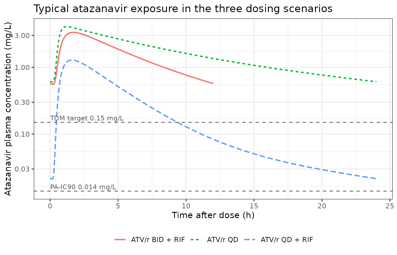
Replicates Figure 4 of Kengo 2025: typical atazanavir plasma concentration-time profiles in the three dosing scenarios, over one steady-state dosing interval.
The paper’s Figure 4 draws the same three curves for a typical 61 kg individual from its simulation reference cohort; the curves here are drawn at the model’s own reference of 42 kg fat-free mass, so they are the published typical values without an additional cohort assumption. The ordering and separation reproduce: ATV/r once daily alone sits highest, adding rifampicin collapses the profile below the 0.15 mg/L therapeutic-drug-monitoring target across the whole interval, and twice-daily ATV/r with rifampicin returns the trough to the once-daily-alone level.
pct <- function(d, col) {
  d |>
    dplyr::mutate(tad = time - last_dose_time) |>
    dplyr::group_by(treatment, tad) |>
    dplyr::summarise(
      lo = stats::quantile(.data[[col]], 0.05),
      mid = stats::median(.data[[col]]),
      hi = stats::quantile(.data[[col]], 0.95),
      .groups = "drop"
    ) |>
    dplyr::mutate(matrix = col)
}

dplyr::bind_rows(pct(sim_atv, "Cc"), pct(sim_atv, "Cpbmc")) |>
  dplyr::mutate(matrix = factor(matrix, c("Cpbmc", "Cc"),
                                c("Intracellular (PBMC)", "Plasma"))) |>
  ggplot2::ggplot(ggplot2::aes(tad, mid, colour = treatment, fill = treatment)) +
  ggplot2::geom_ribbon(ggplot2::aes(ymin = lo, ymax = hi), alpha = 0.15, colour = NA) +
  ggplot2::geom_line(linewidth = 0.7) +
  ggplot2::facet_wrap(~matrix, ncol = 1, scales = "free_y") +
  ggplot2::scale_y_log10() +
  ggplot2::labs(x = "Time after dose (h)", y = "Atazanavir concentration (mg/L)",
                colour = NULL, fill = NULL) +
  ggplot2::theme_bw() +
  ggplot2::theme(legend.position = "bottom")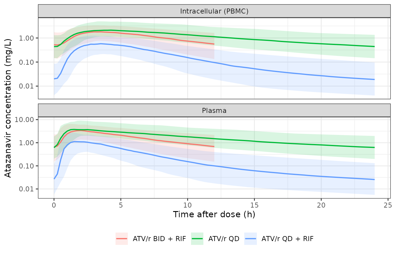
In the manner of Figure 1 of Kengo 2025: simulated plasma (bottom) and intracellular PBMC (top) atazanavir concentrations. The paper’s panel overlays observed data, which are not distributed with the article; percentiles of the simulated cohort are shown instead.
dplyr::bind_rows(pct(sim_rtv, "Cc"), pct(sim_rtv, "Cpbmc")) |>
  dplyr::mutate(matrix = factor(matrix, c("Cpbmc", "Cc"),
                                c("Intracellular (PBMC)", "Plasma"))) |>
  ggplot2::ggplot(ggplot2::aes(tad, mid, colour = treatment, fill = treatment)) +
  ggplot2::geom_ribbon(ggplot2::aes(ymin = lo, ymax = hi), alpha = 0.15, colour = NA) +
  ggplot2::geom_line(linewidth = 0.7) +
  ggplot2::facet_wrap(~matrix, ncol = 1, scales = "free_y") +
  ggplot2::scale_y_log10() +
  ggplot2::labs(x = "Time after dose (h)", y = "Ritonavir concentration (mg/L)",
                colour = NULL, fill = NULL) +
  ggplot2::theme_bw() +
  ggplot2::theme(legend.position = "bottom")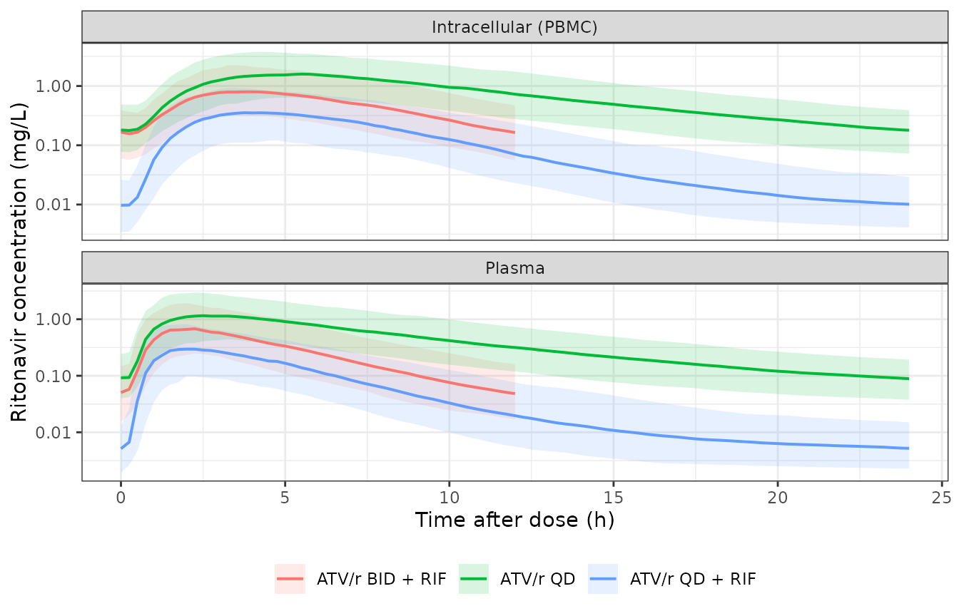
In the manner of Figure 2 of Kengo 2025: simulated plasma (bottom) and intracellular PBMC (top) ritonavir concentrations.
Ritonavir’s intracellular panel sits above its plasma panel, atazanavir’s below – the visual signature of the two pseudo-partition coefficients (1.68 and 0.653) verified numerically above.
troughs <- sim_atv |>
  dplyr::group_by(id, treatment) |>
  dplyr::slice_max(time, n = 1, with_ties = FALSE) |>
  dplyr::ungroup() |>
  dplyr::select(id, treatment, ctrough = Cc, FFM, WT)

troughs |>
  ggplot2::ggplot(ggplot2::aes(treatment, ctrough, fill = treatment)) +
  ggplot2::geom_boxplot(outlier.size = 0.6, alpha = 0.7) +
  ggplot2::geom_hline(yintercept = 0.15, linetype = "dashed", colour = "blue") +
  ggplot2::geom_hline(yintercept = 0.014, linetype = "dashed", colour = "red") +
  ggplot2::scale_y_log10() +
  ggplot2::labs(x = NULL, y = "Atazanavir trough concentration (mg/L)",
                title = "Blue dashed: 0.15 mg/L TDM target. Red dashed: 0.014 mg/L PA-IC90.") +
  ggplot2::theme_bw() +
  ggplot2::theme(legend.position = "none")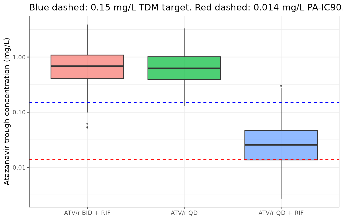
In the manner of Figure 3 of Kengo 2025: simulated atazanavir trough plasma concentrations by dosing scenario.
PKNCA validation
Steady-state non-compartmental analysis over the final dosing interval of each arm, grouped by treatment so the arms are never pooled.
# Time is shifted to time-after-the-last-dose, so each interval runs [0, tau]
# with a measured time-zero record. Two reasons: it gives PKNCA the mandatory
# time-zero point without a defensive row, and PKNCA 0.12.1's pk.nca() hands
# pk.calc.ctrough() a time vector already expressed relative to the dose while
# leaving the interval `end` on the original scale, so an absolute-time
# interval silently returns ctrough = NA. The cross-check below would catch
# that, but shifting avoids it outright.
nca_for <- function(sim, drug_dose) {
  conc <- sim |>
    dplyr::filter(!is.na(Cc)) |>
    dplyr::mutate(tad = time - last_dose_time) |>
    dplyr::select(id, treatment, tad, Cc, tau)

  dose <- conc |>
    dplyr::group_by(id, treatment) |>
    dplyr::summarise(tad = 0, tau = tau[1], .groups = "drop") |>
    dplyr::mutate(amt = drug_dose)

  conc_obj <- PKNCA::PKNCAconc(conc, Cc ~ tad | treatment + id,
                               concu = "mg/L", timeu = "h")
  dose_obj <- PKNCA::PKNCAdose(dose, amt ~ tad | treatment + id, doseu = "mg")

  intervals <- dose |>
    dplyr::distinct(treatment, tau) |>
    dplyr::transmute(
      treatment, start = 0, end = tau,
      cmax = TRUE, tmax = TRUE, cmin = TRUE, auclast = TRUE, cav = TRUE,
      ctrough = TRUE
    ) |>
    dplyr::distinct()

  PKNCA::pk.nca(PKNCA::PKNCAdata(conc_obj, dose_obj, intervals = intervals))
}

nca_atv <- nca_for(sim_atv, 300)
nca_rtv <- nca_for(sim_rtv, 100)

summarise_nca <- function(res, drug) {
  as.data.frame(res) |>
    dplyr::filter(PPTESTCD %in% c("cmax", "tmax", "cmin", "auclast", "cav", "ctrough")) |>
    dplyr::group_by(treatment, PPTESTCD) |>
    dplyr::summarise(value = stats::median(PPORRES, na.rm = TRUE), .groups = "drop") |>
    tidyr::pivot_wider(names_from = PPTESTCD, values_from = value) |>
    dplyr::mutate(Drug = drug)
}

nca_tbl <- dplyr::bind_rows(
  summarise_nca(nca_atv, "Atazanavir"),
  summarise_nca(nca_rtv, "Ritonavir")
)

knitr::kable(
  nca_tbl |>
    dplyr::select(Drug, treatment, cmax, tmax, cmin, ctrough, cav, auclast) |>
    dplyr::rename(
      "Scenario" = treatment,
      "Cmax (mg/L)" = cmax,
      "Tmax (h)" = tmax,
      "Cmin (mg/L)" = cmin,
      "Ctrough (mg/L)" = ctrough,
      "Cav (mg/L)" = cav,
      "AUC0-tau (mg*h/L)" = auclast
    ),
  digits = 4,
  caption = "Median steady-state NCA parameters over the final dosing interval (200 simulated participants per arm)."
)| Drug | Scenario | Cmax (mg/L) | Tmax (h) | Cmin (mg/L) | Ctrough (mg/L) | Cav (mg/L) | AUC0-tau (mg*h/L) |
|---|---|---|---|---|---|---|---|
| Atazanavir | ATV/r BID + RIF | 3.6468 | 1.75 | 0.5514 | 0.6853 | 1.7382 | 20.8590 |
| Atazanavir | ATV/r QD | 4.1533 | 1.50 | 0.5331 | 0.6250 | 1.8346 | 44.0303 |
| Atazanavir | ATV/r QD + RIF | 1.2447 | 1.75 | 0.0208 | 0.0255 | 0.2780 | 6.6709 |
| Ritonavir | ATV/r BID + RIF | 0.7171 | 2.00 | 0.0371 | 0.0483 | 0.2869 | 3.4424 |
| Ritonavir | ATV/r QD | 1.2072 | 2.50 | 0.0779 | 0.0887 | 0.4365 | 10.4754 |
| Ritonavir | ATV/r QD + RIF | 0.3215 | 2.25 | 0.0047 | 0.0052 | 0.0713 | 1.7120 |
Kengo 2025 reports no non-compartmental table of its own – the
companion non-compartmental analysis of the DERIVE trial is its
reference 8, which was not available when this model was built – so
there is no published Cmax / AUC / half-life row to place beside these.
The paper’s own quantitative simulation output is the trough
target-attainment table reproduced next, and
nlmixr2lib::ncaComparisonTable() is therefore not used.
# The NCA interval must be the full dosing interval, and PKNCA's ctrough
# (concentration at the interval end) must equal the trough read directly off
# the solved grid. The conc frame carries no dose record at the interval end,
# so ctrough reads the pre-next-dose value rather than a post-dose one.
# PKNCA returns the grouping columns with its own types, so both sides are
# coerced before the join rather than relying on them matching.
nca_ctrough <- as.data.frame(nca_atv) |>
  dplyr::filter(PPTESTCD == "ctrough") |>
  dplyr::transmute(
    treatment = as.character(treatment),
    id = as.integer(as.character(id)),
    ctrough_nca = PPORRES
  )

ctrough_check <- troughs |>
  dplyr::transmute(treatment = as.character(treatment), id = as.integer(id), ctrough) |>
  dplyr::inner_join(nca_ctrough, by = c("treatment", "id"))

cat(sprintf(
  "ctrough cross-check: %d of %d subjects matched; max relative difference %.3g\n",
  nrow(ctrough_check), 3 * n_per_arm,
  max(abs(ctrough_check$ctrough_nca - ctrough_check$ctrough) / ctrough_check$ctrough)
))
#> ctrough cross-check: 600 of 600 subjects matched; max relative difference 0

stopifnot(
  nrow(ctrough_check) == 3 * n_per_arm,
  max(abs(ctrough_check$ctrough_nca - ctrough_check$ctrough) /
        ctrough_check$ctrough) < 1e-6
)
Comparison against the published simulation
Kengo 2025 Results 3.7 reports the proportion of simulated individuals reaching each atazanavir trough target in each of the three scenarios. Those percentages come from the authors’ own Monte Carlo run over a reference cohort of 1225 in-silico individuals built from previous African HIV/TB studies – a broader and lighter population than DERIVE (its typical individual weighs 61 kg against DERIVE’s 67 kg median, and it spans the WHO weight bands). The virtual cohort here is built on the DERIVE demographics of Table 1, which are the only demographics the article tabulates, so close agreement is not guaranteed. In the event every cell lands within about two percentage points of the published value; the assertions that follow are nevertheless written on the paper’s qualitative conclusions rather than on those percentages, because a 200-participant arm carries a Monte Carlo standard error of a few percent and the tails of a random cohort are not reproducible across rxode2 builds.
attainment <- troughs |>
  dplyr::group_by(treatment) |>
  dplyr::summarise(
    `> 0.014 mg/L` = 100 * mean(ctrough > 0.014),
    `> 0.15 mg/L` = 100 * mean(ctrough > 0.15),
    .groups = "drop"
  ) |>
  dplyr::mutate(
    `Published > 0.014 mg/L` = c(100, 99, 72.8)[match(treatment,
      c("ATV/r QD", "ATV/r BID + RIF", "ATV/r QD + RIF"))],
    `Published > 0.15 mg/L` = c(95.4, 94, 2.83)[match(treatment,
      c("ATV/r QD", "ATV/r BID + RIF", "ATV/r QD + RIF"))]
  )

knitr::kable(
  attainment |>
    dplyr::select(Scenario = treatment,
                  `Simulated > 0.014 mg/L (%)` = `> 0.014 mg/L`,
                  `Published > 0.014 mg/L (%)` = `Published > 0.014 mg/L`,
                  `Simulated > 0.15 mg/L (%)` = `> 0.15 mg/L`,
                  `Published > 0.15 mg/L (%)` = `Published > 0.15 mg/L`),
  digits = 1,
  caption = "Atazanavir trough target attainment against Kengo 2025 Results 3.7."
)| Scenario | Simulated > 0.014 mg/L (%) | Published > 0.014 mg/L (%) | Simulated > 0.15 mg/L (%) | Published > 0.15 mg/L (%) |
|---|---|---|---|---|
| ATV/r BID + RIF | 100.0 | 99.0 | 95.0 | 94.0 |
| ATV/r QD | 100.0 | 100.0 | 96.5 | 95.4 |
| ATV/r QD + RIF | 73.5 | 72.8 | 4.5 | 2.8 |
get_att <- function(scn, col) attainment[[col]][attainment$treatment == scn]

# The paper's three qualitative conclusions, asserted as ordering facts that are
# robust to the cohort difference described above. Exact percentages are NOT
# asserted: the published run used a different, broader reference cohort, and a
# 200-participant arm carries a Monte Carlo standard error of a few percent.
stopifnot(
  # 1. ATV/r alone: essentially everyone clears the PA-IC90, and the large
  #    majority clear the 0.15 mg/L TDM target.
  get_att("ATV/r QD", "> 0.014 mg/L") > 99,
  get_att("ATV/r QD", "> 0.15 mg/L") > 85,
  # 2. Adding rifampicin to once-daily ATV/r collapses attainment of the
  #    0.15 mg/L target (published 2.83%) and erodes the PA-IC90 (published
  #    72.8%).
  get_att("ATV/r QD + RIF", "> 0.15 mg/L") < 15,
  get_att("ATV/r QD + RIF", "> 0.014 mg/L") < 90,
  # 3. Doubling the dosing frequency restores both (published 99% and 94%).
  get_att("ATV/r BID + RIF", "> 0.014 mg/L") > 95,
  get_att("ATV/r BID + RIF", "> 0.15 mg/L") > 75,
  # 4. And the restored trough is comparable to ATV/r alone, which is the
  #    paper's conclusion. Compare medians, not extremes.
  {
    med <- troughs |>
      dplyr::group_by(treatment) |>
      dplyr::summarise(m = stats::median(ctrough), .groups = "drop")
    r <- med$m[med$treatment == "ATV/r BID + RIF"] / med$m[med$treatment == "ATV/r QD"]
    r > 0.5 && r < 2
  }
)
The three conclusions reproduce, and the agreement is closer than the cohort difference entitles it to be: every cell of the table is within about two percentage points of the published value, including the collapse of 0.15 mg/L attainment to the low single digits when rifampicin is added to once-daily ATV/r, and its recovery to the mid-nineties when the dosing frequency is doubled. That the two cohorts agree this well is itself informative – trough attainment in this model is driven overwhelmingly by the regimen covariates and the between-subject and between-occasion random effects, not by the size distribution, because fat-free mass enters only through a 0.75-power allometric term on clearance.
The unboosted-atazanavir model (ACTG A5231)
Kengo_2025_atazanavir_a5231 is the same structure
re-fitted to atazanavir given without ritonavir. It has
no PBMC compartment because A5231 collected no intracellular samples.
The checks below confirm the two estimated covariate effects and the
slower absorption against Table S3.
make_a5231_arm <- function(dose, rif, label, id_offset, rtv_present = 0) {
  ii <- 12
  n_dose <- t_end / ii
  ids <- id_offset + subjects$subject
  # This model encodes the Savic delay as an EXPLICIT 11-compartment chain, so
  # the dose is administered to `transit1`, not to `depot`. See the model
  # file's ODE-block comment and the Errata below for why it cannot use the
  # closed-form transit() density the two DERIVE models use.
  dosing <- tidyr::expand_grid(id = ids, time = seq(0, ii * (n_dose - 1), by = ii)) |>
    dplyr::mutate(amt = dose, evid = 1L, cmt = "transit1")
  # This model has a SINGLE endpoint, so observations are written on the ODE
  # state "central" and rxode2 returns the algebraic Cc alongside it. That is
  # the opposite of the two-endpoint DERIVE models above, where naming an ODE
  # state on the observation row is what fails.
  obs <- tidyr::expand_grid(id = ids, time = seq(ii * (n_dose - 1), t_end, by = 0.02)) |>
    dplyr::mutate(amt = NA_real_, evid = 0L, cmt = "central")
  dplyr::bind_rows(dosing, obs) |>
    dplyr::mutate(
      FFM = 42, CONMED_RIF = rif, CONMED_RTV = rtv_present, SELFADMIN = 0,
      # This model carries six occasions rather than eight.
      OCC = as.integer(floor(time / ii)) %% 6L + 1L,
      treatment = label, tau = ii, last_dose_time = ii * (n_dose - 1)
    ) |>
    dplyr::arrange(id, time, dplyr::desc(evid))
}

a5231_arms <- dplyr::bind_rows(
  make_a5231_arm(300, 0, "ATV 300 BID (boosted reference)", 0L, rtv_present = 1),
  make_a5231_arm(300, 0, "ATV 300 BID, no RTV", 1000L),
  make_a5231_arm(300, 1, "ATV 300 BID, no RTV + RIF", 2000L),
  make_a5231_arm(400, 1, "ATV 400 BID, no RTV + RIF", 3000L)
) |>
  dplyr::filter(id %in% c(1L, 1001L, 2001L, 3001L))

sim_a5231 <- rxode2::rxSolve(
  rxode2::zeroRe(a5231), events = a5231_arms,
  keep = c("treatment", "tau", "last_dose_time"), useLinCmt = FALSE
) |>
  as.data.frame() |>
  dplyr::filter(!is.na(Cc))
#> ℹ parameter labels from comments will be replaced by 'label()'
#> Warning: some etas defaulted to non-mu referenced, possible parsing error: etaiov_ka_1, etaiov_ka_2, etaiov_ka_3, etaiov_ka_4, etaiov_ka_5, etaiov_ka_6, etaiov_mtt_1, etaiov_mtt_2, etaiov_mtt_3, etaiov_mtt_4, etaiov_mtt_5, etaiov_mtt_6, etaiov_fdepot_1, etaiov_fdepot_2, etaiov_fdepot_3, etaiov_fdepot_4, etaiov_fdepot_5, etaiov_fdepot_6
#> as a work-around try putting the mu-referenced expression on a simple line
#> Warning: some etas defaulted to non-mu referenced, possible parsing error: etaiov_ka_1, etaiov_ka_2, etaiov_ka_3, etaiov_ka_4, etaiov_ka_5, etaiov_ka_6, etaiov_mtt_1, etaiov_mtt_2, etaiov_mtt_3, etaiov_mtt_4, etaiov_mtt_5, etaiov_mtt_6, etaiov_fdepot_1, etaiov_fdepot_2, etaiov_fdepot_3, etaiov_fdepot_4, etaiov_fdepot_5, etaiov_fdepot_6
#> as a work-around try putting the mu-referenced expression on a simple line
#> ℹ omega/sigma items treated as zero: 'etalcl', 'etaiov_ka_1', 'etaiov_ka_2', 'etaiov_ka_3', 'etaiov_ka_4', 'etaiov_ka_5', 'etaiov_ka_6', 'etaiov_mtt_1', 'etaiov_mtt_2', 'etaiov_mtt_3', 'etaiov_mtt_4', 'etaiov_mtt_5', 'etaiov_mtt_6', 'etaiov_fdepot_1', 'etaiov_fdepot_2', 'etaiov_fdepot_3', 'etaiov_fdepot_4', 'etaiov_fdepot_5', 'etaiov_fdepot_6'
#> Warning: multi-subject simulation without without 'omega'

a5231_auc <- sim_a5231 |>
  dplyr::group_by(treatment) |>
  dplyr::summarise(auc_tau = trap(time, Cc), tmax = time[which.max(Cc)] - last_dose_time[1],
                   .groups = "drop")

ref_auc <- a5231_auc$auc_tau[a5231_auc$treatment == "ATV 300 BID (boosted reference)"]
noRtv_auc <- a5231_auc$auc_tau[a5231_auc$treatment == "ATV 300 BID, no RTV"]
rif_auc <- a5231_auc$auc_tau[a5231_auc$treatment == "ATV 300 BID, no RTV + RIF"]

a5231_check <- dplyr::tibble(
  Comparison = c("Absence of ritonavir (AUC ratio)",
                 "Rifampicin on bioavailability (AUC ratio)",
                 "Dose proportionality 400 vs 300 mg (AUC ratio)"),
  Simulated = c(
    noRtv_auc / ref_auc,
    rif_auc / noRtv_auc,
    a5231_auc$auc_tau[a5231_auc$treatment == "ATV 400 BID, no RTV + RIF"] / rif_auc
  ),
  `Expected from Table S3` = c(1 / 2.13, 1 - 0.553, 400 / 300)
) |>
  dplyr::mutate(`% diff` = 100 * (Simulated / `Expected from Table S3` - 1))

knitr::kable(a5231_check, digits = 4,
caption = "Unboosted-atazanavir model against supplementary Table S3.")| Comparison | Simulated | Expected from Table S3 | % diff |
|---|---|---|---|
| Absence of ritonavir (AUC ratio) | 0.4695 | 0.4695 | 0 |
| Rifampicin on bioavailability (AUC ratio) | 0.4470 | 0.4470 | 0 |
| Dose proportionality 400 vs 300 mg (AUC ratio) | 1.3333 | 1.3333 | 0 |
stopifnot(max(abs(a5231_check$`% diff`)) < 0.5)

# Absorption is slower in A5231 than in DERIVE: MTT 1.38 h against 0.499 h, so
# Tmax must be later. The DERIVE comparator is the ATV/r QD typical profile.
tmax_derive <- sim_atv_typ |>
  dplyr::filter(treatment == "ATV/r QD") |>
  dplyr::summarise(t = time[which.max(Cc)] - last_dose_time[1]) |>
  dplyr::pull(t)
tmax_a5231 <- a5231_auc$tmax[a5231_auc$treatment == "ATV 300 BID, no RTV"]
cat(sprintf("Typical Tmax: DERIVE %.2f h, A5231 %.2f h\n", tmax_derive, tmax_a5231))
#> Typical Tmax: DERIVE 1.22 h, A5231 2.30 h
stopifnot(tmax_a5231 > tmax_derive)
The model is linear in dose, so the 400 mg arm scales exactly 4/3 – Table S3 carries no dose-dependent term, and A5231’s two rifampicin periods differ only in the atazanavir dose.
Absorption mass balance
Every model here has an absorption delay, and a delayed-input
encoding can fail silently: if the input rate evaluates to zero
the solver returns all-zero concentrations with no error and no
NA, and every ratio-based check above still “passes”
because it divides one zero by another. The check that cannot be fooled
is steady-state mass balance – over one dosing interval at steady state,
cl * AUCtau must equal Dose * F exactly. It
catches a dead absorption pathway (ratio 0) and the opposite failure of
a dose that arrives twice, once through the delay and once as an
un-suppressed bolus (ratio 2).
This gate is run on typical values (zeroRe()), where the
identity is exact rather than a Monte Carlo approximation, over every
regimen arm of all three models.
mass_balance <- function(mod, dose, ii, dose_cmt, covs, label,
                         two_endpoint = TRUE) {
  t_horizon <- 1440
  ev <- rxode2::et(amt = dose, cmt = dose_cmt, ii = ii,
                   addl = t_horizon / ii - 1) |>
    rxode2::et(seq(0, t_horizon, by = 0.05), cmt = "central")
  d <- as.data.frame(ev)
  # The two DERIVE models have two endpoints, so their observation rows must
  # nominate one; the single-endpoint A5231 model must not carry a dvid column.
  if (two_endpoint) {
    d$dvid <- ifelse(is.na(d$amt), 1L, NA_integer_)
  }
  for (nm in names(covs)) d[[nm]] <- covs[[nm]]
  s <- rxode2::rxSolve(mod, d, returnType = "data.frame", useLinCmt = FALSE)
  last <- s[s$time >= t_horizon - ii & s$time <= t_horizon, ]
  auc <- trap(last$time, last$Cc)
  dplyr::tibble(
    Model = label, `cl (L/h)` = last$cl[1], F = last$fdepot[1],
    `AUCtau` = auc, `cl*AUCtau/(Dose*F)` = last$cl[1] * auc / (dose * last$fdepot[1])
  )
}

atv_cov <- function(rif, bid) {
  list(FFM = 42, CONMED_RIF = rif, REGI_BID = bid, OCC = 1, SELFADMIN = 0)
}

mb <- dplyr::bind_rows(
  mass_balance(rxode2::zeroRe(atv), 300, 24, "depot", atv_cov(0, 0),
               "atazanavir, ATV/r QD"),
  mass_balance(rxode2::zeroRe(atv), 300, 24, "depot", atv_cov(1, 0),
               "atazanavir, ATV/r QD + RIF"),
  mass_balance(rxode2::zeroRe(atv), 300, 12, "depot", atv_cov(1, 1),
               "atazanavir, ATV/r BID + RIF"),
  mass_balance(rxode2::zeroRe(rtv), 100, 24, "depot",
               list(FFM = 42, CONMED_RIF = 0, REGI_BID = 0, OCC = 1),
               "ritonavir, ATV/r QD"),
  mass_balance(rxode2::zeroRe(rtv), 100, 24, "depot",
               list(FFM = 42, CONMED_RIF = 1, REGI_BID = 0, OCC = 1),
               "ritonavir, ATV/r QD + RIF"),
  mass_balance(rxode2::zeroRe(rtv), 100, 12, "depot",
               list(FFM = 42, CONMED_RIF = 1, REGI_BID = 1, OCC = 1),
               "ritonavir, ATV/r BID + RIF"),
  mass_balance(rxode2::zeroRe(a5231), 300, 12, "transit1",
               list(FFM = 42, CONMED_RIF = 0, CONMED_RTV = 0, OCC = 1, SELFADMIN = 0),
               "A5231, ATV 300 BID no RIF", two_endpoint = FALSE),
  mass_balance(rxode2::zeroRe(a5231), 300, 12, "transit1",
               list(FFM = 42, CONMED_RIF = 1, CONMED_RTV = 0, OCC = 1, SELFADMIN = 0),
               "A5231, ATV 300 BID + RIF", two_endpoint = FALSE),
  mass_balance(rxode2::zeroRe(a5231), 400, 12, "transit1",
               list(FFM = 42, CONMED_RIF = 1, CONMED_RTV = 0, OCC = 1, SELFADMIN = 0),
               "A5231, ATV 400 BID + RIF", two_endpoint = FALSE)
)
#> ℹ parameter labels from comments will be replaced by 'label()'
#> Warning: some etas defaulted to non-mu referenced, possible parsing error: etabvv_cl_1, etabvv_cl_2, etabvv_cl_3, etabvv_cl_4, etaiov_ka_1, etaiov_ka_2, etaiov_ka_3, etaiov_ka_4, etaiov_ka_5, etaiov_ka_6, etaiov_ka_7, etaiov_ka_8, etaiov_mtt_1, etaiov_mtt_2, etaiov_mtt_3, etaiov_mtt_4, etaiov_mtt_5, etaiov_mtt_6, etaiov_mtt_7, etaiov_mtt_8, etaiov_fdepot_1, etaiov_fdepot_2, etaiov_fdepot_3, etaiov_fdepot_4, etaiov_fdepot_5, etaiov_fdepot_6, etaiov_fdepot_7, etaiov_fdepot_8
#> as a work-around try putting the mu-referenced expression on a simple line
#> Warning: some etas defaulted to non-mu referenced, possible parsing error: etabvv_cl_1, etabvv_cl_2, etabvv_cl_3, etabvv_cl_4, etaiov_ka_1, etaiov_ka_2, etaiov_ka_3, etaiov_ka_4, etaiov_ka_5, etaiov_ka_6, etaiov_ka_7, etaiov_ka_8, etaiov_mtt_1, etaiov_mtt_2, etaiov_mtt_3, etaiov_mtt_4, etaiov_mtt_5, etaiov_mtt_6, etaiov_mtt_7, etaiov_mtt_8, etaiov_fdepot_1, etaiov_fdepot_2, etaiov_fdepot_3, etaiov_fdepot_4, etaiov_fdepot_5, etaiov_fdepot_6, etaiov_fdepot_7, etaiov_fdepot_8
#> as a work-around try putting the mu-referenced expression on a simple line
#> ℹ omega/sigma items treated as zero: 'etalcl', 'etabvv_cl_1', 'etabvv_cl_2', 'etabvv_cl_3', 'etabvv_cl_4', 'etaiov_ka_1', 'etaiov_ka_2', 'etaiov_ka_3', 'etaiov_ka_4', 'etaiov_ka_5', 'etaiov_ka_6', 'etaiov_ka_7', 'etaiov_ka_8', 'etaiov_mtt_1', 'etaiov_mtt_2', 'etaiov_mtt_3', 'etaiov_mtt_4', 'etaiov_mtt_5', 'etaiov_mtt_6', 'etaiov_mtt_7', 'etaiov_mtt_8', 'etaiov_fdepot_1', 'etaiov_fdepot_2', 'etaiov_fdepot_3', 'etaiov_fdepot_4', 'etaiov_fdepot_5', 'etaiov_fdepot_6', 'etaiov_fdepot_7', 'etaiov_fdepot_8'
#> ℹ parameter labels from comments will be replaced by 'label()'
#> Warning: some etas defaulted to non-mu referenced, possible parsing error: etabvv_cl_1, etabvv_cl_2, etabvv_cl_3, etabvv_cl_4, etaiov_ka_1, etaiov_ka_2, etaiov_ka_3, etaiov_ka_4, etaiov_ka_5, etaiov_ka_6, etaiov_ka_7, etaiov_ka_8, etaiov_mtt_1, etaiov_mtt_2, etaiov_mtt_3, etaiov_mtt_4, etaiov_mtt_5, etaiov_mtt_6, etaiov_mtt_7, etaiov_mtt_8, etaiov_fdepot_1, etaiov_fdepot_2, etaiov_fdepot_3, etaiov_fdepot_4, etaiov_fdepot_5, etaiov_fdepot_6, etaiov_fdepot_7, etaiov_fdepot_8
#> as a work-around try putting the mu-referenced expression on a simple line
#> Warning: some etas defaulted to non-mu referenced, possible parsing error: etabvv_cl_1, etabvv_cl_2, etabvv_cl_3, etabvv_cl_4, etaiov_ka_1, etaiov_ka_2, etaiov_ka_3, etaiov_ka_4, etaiov_ka_5, etaiov_ka_6, etaiov_ka_7, etaiov_ka_8, etaiov_mtt_1, etaiov_mtt_2, etaiov_mtt_3, etaiov_mtt_4, etaiov_mtt_5, etaiov_mtt_6, etaiov_mtt_7, etaiov_mtt_8, etaiov_fdepot_1, etaiov_fdepot_2, etaiov_fdepot_3, etaiov_fdepot_4, etaiov_fdepot_5, etaiov_fdepot_6, etaiov_fdepot_7, etaiov_fdepot_8
#> as a work-around try putting the mu-referenced expression on a simple line
#> ℹ omega/sigma items treated as zero: 'etalcl', 'etabvv_cl_1', 'etabvv_cl_2', 'etabvv_cl_3', 'etabvv_cl_4', 'etaiov_ka_1', 'etaiov_ka_2', 'etaiov_ka_3', 'etaiov_ka_4', 'etaiov_ka_5', 'etaiov_ka_6', 'etaiov_ka_7', 'etaiov_ka_8', 'etaiov_mtt_1', 'etaiov_mtt_2', 'etaiov_mtt_3', 'etaiov_mtt_4', 'etaiov_mtt_5', 'etaiov_mtt_6', 'etaiov_mtt_7', 'etaiov_mtt_8', 'etaiov_fdepot_1', 'etaiov_fdepot_2', 'etaiov_fdepot_3', 'etaiov_fdepot_4', 'etaiov_fdepot_5', 'etaiov_fdepot_6', 'etaiov_fdepot_7', 'etaiov_fdepot_8'
#> ℹ parameter labels from comments will be replaced by 'label()'
#> Warning: some etas defaulted to non-mu referenced, possible parsing error: etabvv_cl_1, etabvv_cl_2, etabvv_cl_3, etabvv_cl_4, etaiov_ka_1, etaiov_ka_2, etaiov_ka_3, etaiov_ka_4, etaiov_ka_5, etaiov_ka_6, etaiov_ka_7, etaiov_ka_8, etaiov_mtt_1, etaiov_mtt_2, etaiov_mtt_3, etaiov_mtt_4, etaiov_mtt_5, etaiov_mtt_6, etaiov_mtt_7, etaiov_mtt_8, etaiov_fdepot_1, etaiov_fdepot_2, etaiov_fdepot_3, etaiov_fdepot_4, etaiov_fdepot_5, etaiov_fdepot_6, etaiov_fdepot_7, etaiov_fdepot_8
#> as a work-around try putting the mu-referenced expression on a simple line
#> Warning: some etas defaulted to non-mu referenced, possible parsing error: etabvv_cl_1, etabvv_cl_2, etabvv_cl_3, etabvv_cl_4, etaiov_ka_1, etaiov_ka_2, etaiov_ka_3, etaiov_ka_4, etaiov_ka_5, etaiov_ka_6, etaiov_ka_7, etaiov_ka_8, etaiov_mtt_1, etaiov_mtt_2, etaiov_mtt_3, etaiov_mtt_4, etaiov_mtt_5, etaiov_mtt_6, etaiov_mtt_7, etaiov_mtt_8, etaiov_fdepot_1, etaiov_fdepot_2, etaiov_fdepot_3, etaiov_fdepot_4, etaiov_fdepot_5, etaiov_fdepot_6, etaiov_fdepot_7, etaiov_fdepot_8
#> as a work-around try putting the mu-referenced expression on a simple line
#> ℹ omega/sigma items treated as zero: 'etalcl', 'etabvv_cl_1', 'etabvv_cl_2', 'etabvv_cl_3', 'etabvv_cl_4', 'etaiov_ka_1', 'etaiov_ka_2', 'etaiov_ka_3', 'etaiov_ka_4', 'etaiov_ka_5', 'etaiov_ka_6', 'etaiov_ka_7', 'etaiov_ka_8', 'etaiov_mtt_1', 'etaiov_mtt_2', 'etaiov_mtt_3', 'etaiov_mtt_4', 'etaiov_mtt_5', 'etaiov_mtt_6', 'etaiov_mtt_7', 'etaiov_mtt_8', 'etaiov_fdepot_1', 'etaiov_fdepot_2', 'etaiov_fdepot_3', 'etaiov_fdepot_4', 'etaiov_fdepot_5', 'etaiov_fdepot_6', 'etaiov_fdepot_7', 'etaiov_fdepot_8'
#> ℹ parameter labels from comments will be replaced by 'label()'
#> Warning: some etas defaulted to non-mu referenced, possible parsing error: etaiov_ka_1, etaiov_ka_2, etaiov_ka_3, etaiov_ka_4, etaiov_ka_5, etaiov_ka_6, etaiov_ka_7, etaiov_ka_8, etaiov_mtt_1, etaiov_mtt_2, etaiov_mtt_3, etaiov_mtt_4, etaiov_mtt_5, etaiov_mtt_6, etaiov_mtt_7, etaiov_mtt_8, etaiov_fdepot_1, etaiov_fdepot_2, etaiov_fdepot_3, etaiov_fdepot_4, etaiov_fdepot_5, etaiov_fdepot_6, etaiov_fdepot_7, etaiov_fdepot_8
#> as a work-around try putting the mu-referenced expression on a simple line
#> Warning: some etas defaulted to non-mu referenced, possible parsing error: etaiov_ka_1, etaiov_ka_2, etaiov_ka_3, etaiov_ka_4, etaiov_ka_5, etaiov_ka_6, etaiov_ka_7, etaiov_ka_8, etaiov_mtt_1, etaiov_mtt_2, etaiov_mtt_3, etaiov_mtt_4, etaiov_mtt_5, etaiov_mtt_6, etaiov_mtt_7, etaiov_mtt_8, etaiov_fdepot_1, etaiov_fdepot_2, etaiov_fdepot_3, etaiov_fdepot_4, etaiov_fdepot_5, etaiov_fdepot_6, etaiov_fdepot_7, etaiov_fdepot_8
#> as a work-around try putting the mu-referenced expression on a simple line
#> ℹ omega/sigma items treated as zero: 'etalcl', 'etaiov_ka_1', 'etaiov_ka_2', 'etaiov_ka_3', 'etaiov_ka_4', 'etaiov_ka_5', 'etaiov_ka_6', 'etaiov_ka_7', 'etaiov_ka_8', 'etaiov_mtt_1', 'etaiov_mtt_2', 'etaiov_mtt_3', 'etaiov_mtt_4', 'etaiov_mtt_5', 'etaiov_mtt_6', 'etaiov_mtt_7', 'etaiov_mtt_8', 'etaiov_fdepot_1', 'etaiov_fdepot_2', 'etaiov_fdepot_3', 'etaiov_fdepot_4', 'etaiov_fdepot_5', 'etaiov_fdepot_6', 'etaiov_fdepot_7', 'etaiov_fdepot_8'
#> ℹ parameter labels from comments will be replaced by 'label()'
#> Warning: some etas defaulted to non-mu referenced, possible parsing error: etaiov_ka_1, etaiov_ka_2, etaiov_ka_3, etaiov_ka_4, etaiov_ka_5, etaiov_ka_6, etaiov_ka_7, etaiov_ka_8, etaiov_mtt_1, etaiov_mtt_2, etaiov_mtt_3, etaiov_mtt_4, etaiov_mtt_5, etaiov_mtt_6, etaiov_mtt_7, etaiov_mtt_8, etaiov_fdepot_1, etaiov_fdepot_2, etaiov_fdepot_3, etaiov_fdepot_4, etaiov_fdepot_5, etaiov_fdepot_6, etaiov_fdepot_7, etaiov_fdepot_8
#> as a work-around try putting the mu-referenced expression on a simple line
#> Warning: some etas defaulted to non-mu referenced, possible parsing error: etaiov_ka_1, etaiov_ka_2, etaiov_ka_3, etaiov_ka_4, etaiov_ka_5, etaiov_ka_6, etaiov_ka_7, etaiov_ka_8, etaiov_mtt_1, etaiov_mtt_2, etaiov_mtt_3, etaiov_mtt_4, etaiov_mtt_5, etaiov_mtt_6, etaiov_mtt_7, etaiov_mtt_8, etaiov_fdepot_1, etaiov_fdepot_2, etaiov_fdepot_3, etaiov_fdepot_4, etaiov_fdepot_5, etaiov_fdepot_6, etaiov_fdepot_7, etaiov_fdepot_8
#> as a work-around try putting the mu-referenced expression on a simple line
#> ℹ omega/sigma items treated as zero: 'etalcl', 'etaiov_ka_1', 'etaiov_ka_2', 'etaiov_ka_3', 'etaiov_ka_4', 'etaiov_ka_5', 'etaiov_ka_6', 'etaiov_ka_7', 'etaiov_ka_8', 'etaiov_mtt_1', 'etaiov_mtt_2', 'etaiov_mtt_3', 'etaiov_mtt_4', 'etaiov_mtt_5', 'etaiov_mtt_6', 'etaiov_mtt_7', 'etaiov_mtt_8', 'etaiov_fdepot_1', 'etaiov_fdepot_2', 'etaiov_fdepot_3', 'etaiov_fdepot_4', 'etaiov_fdepot_5', 'etaiov_fdepot_6', 'etaiov_fdepot_7', 'etaiov_fdepot_8'
#> ℹ parameter labels from comments will be replaced by 'label()'
#> Warning: some etas defaulted to non-mu referenced, possible parsing error: etaiov_ka_1, etaiov_ka_2, etaiov_ka_3, etaiov_ka_4, etaiov_ka_5, etaiov_ka_6, etaiov_ka_7, etaiov_ka_8, etaiov_mtt_1, etaiov_mtt_2, etaiov_mtt_3, etaiov_mtt_4, etaiov_mtt_5, etaiov_mtt_6, etaiov_mtt_7, etaiov_mtt_8, etaiov_fdepot_1, etaiov_fdepot_2, etaiov_fdepot_3, etaiov_fdepot_4, etaiov_fdepot_5, etaiov_fdepot_6, etaiov_fdepot_7, etaiov_fdepot_8
#> as a work-around try putting the mu-referenced expression on a simple line
#> Warning: some etas defaulted to non-mu referenced, possible parsing error: etaiov_ka_1, etaiov_ka_2, etaiov_ka_3, etaiov_ka_4, etaiov_ka_5, etaiov_ka_6, etaiov_ka_7, etaiov_ka_8, etaiov_mtt_1, etaiov_mtt_2, etaiov_mtt_3, etaiov_mtt_4, etaiov_mtt_5, etaiov_mtt_6, etaiov_mtt_7, etaiov_mtt_8, etaiov_fdepot_1, etaiov_fdepot_2, etaiov_fdepot_3, etaiov_fdepot_4, etaiov_fdepot_5, etaiov_fdepot_6, etaiov_fdepot_7, etaiov_fdepot_8
#> as a work-around try putting the mu-referenced expression on a simple line
#> ℹ omega/sigma items treated as zero: 'etalcl', 'etaiov_ka_1', 'etaiov_ka_2', 'etaiov_ka_3', 'etaiov_ka_4', 'etaiov_ka_5', 'etaiov_ka_6', 'etaiov_ka_7', 'etaiov_ka_8', 'etaiov_mtt_1', 'etaiov_mtt_2', 'etaiov_mtt_3', 'etaiov_mtt_4', 'etaiov_mtt_5', 'etaiov_mtt_6', 'etaiov_mtt_7', 'etaiov_mtt_8', 'etaiov_fdepot_1', 'etaiov_fdepot_2', 'etaiov_fdepot_3', 'etaiov_fdepot_4', 'etaiov_fdepot_5', 'etaiov_fdepot_6', 'etaiov_fdepot_7', 'etaiov_fdepot_8'
#> ℹ parameter labels from comments will be replaced by 'label()'
#> Warning: some etas defaulted to non-mu referenced, possible parsing error: etaiov_ka_1, etaiov_ka_2, etaiov_ka_3, etaiov_ka_4, etaiov_ka_5, etaiov_ka_6, etaiov_mtt_1, etaiov_mtt_2, etaiov_mtt_3, etaiov_mtt_4, etaiov_mtt_5, etaiov_mtt_6, etaiov_fdepot_1, etaiov_fdepot_2, etaiov_fdepot_3, etaiov_fdepot_4, etaiov_fdepot_5, etaiov_fdepot_6
#> as a work-around try putting the mu-referenced expression on a simple line
#> Warning: some etas defaulted to non-mu referenced, possible parsing error: etaiov_ka_1, etaiov_ka_2, etaiov_ka_3, etaiov_ka_4, etaiov_ka_5, etaiov_ka_6, etaiov_mtt_1, etaiov_mtt_2, etaiov_mtt_3, etaiov_mtt_4, etaiov_mtt_5, etaiov_mtt_6, etaiov_fdepot_1, etaiov_fdepot_2, etaiov_fdepot_3, etaiov_fdepot_4, etaiov_fdepot_5, etaiov_fdepot_6
#> as a work-around try putting the mu-referenced expression on a simple line
#> ℹ omega/sigma items treated as zero: 'etalcl', 'etaiov_ka_1', 'etaiov_ka_2', 'etaiov_ka_3', 'etaiov_ka_4', 'etaiov_ka_5', 'etaiov_ka_6', 'etaiov_mtt_1', 'etaiov_mtt_2', 'etaiov_mtt_3', 'etaiov_mtt_4', 'etaiov_mtt_5', 'etaiov_mtt_6', 'etaiov_fdepot_1', 'etaiov_fdepot_2', 'etaiov_fdepot_3', 'etaiov_fdepot_4', 'etaiov_fdepot_5', 'etaiov_fdepot_6'
#> ℹ parameter labels from comments will be replaced by 'label()'
#> Warning: some etas defaulted to non-mu referenced, possible parsing error: etaiov_ka_1, etaiov_ka_2, etaiov_ka_3, etaiov_ka_4, etaiov_ka_5, etaiov_ka_6, etaiov_mtt_1, etaiov_mtt_2, etaiov_mtt_3, etaiov_mtt_4, etaiov_mtt_5, etaiov_mtt_6, etaiov_fdepot_1, etaiov_fdepot_2, etaiov_fdepot_3, etaiov_fdepot_4, etaiov_fdepot_5, etaiov_fdepot_6
#> as a work-around try putting the mu-referenced expression on a simple line
#> Warning: some etas defaulted to non-mu referenced, possible parsing error: etaiov_ka_1, etaiov_ka_2, etaiov_ka_3, etaiov_ka_4, etaiov_ka_5, etaiov_ka_6, etaiov_mtt_1, etaiov_mtt_2, etaiov_mtt_3, etaiov_mtt_4, etaiov_mtt_5, etaiov_mtt_6, etaiov_fdepot_1, etaiov_fdepot_2, etaiov_fdepot_3, etaiov_fdepot_4, etaiov_fdepot_5, etaiov_fdepot_6
#> as a work-around try putting the mu-referenced expression on a simple line
#> ℹ omega/sigma items treated as zero: 'etalcl', 'etaiov_ka_1', 'etaiov_ka_2', 'etaiov_ka_3', 'etaiov_ka_4', 'etaiov_ka_5', 'etaiov_ka_6', 'etaiov_mtt_1', 'etaiov_mtt_2', 'etaiov_mtt_3', 'etaiov_mtt_4', 'etaiov_mtt_5', 'etaiov_mtt_6', 'etaiov_fdepot_1', 'etaiov_fdepot_2', 'etaiov_fdepot_3', 'etaiov_fdepot_4', 'etaiov_fdepot_5', 'etaiov_fdepot_6'
#> ℹ parameter labels from comments will be replaced by 'label()'
#> Warning: some etas defaulted to non-mu referenced, possible parsing error: etaiov_ka_1, etaiov_ka_2, etaiov_ka_3, etaiov_ka_4, etaiov_ka_5, etaiov_ka_6, etaiov_mtt_1, etaiov_mtt_2, etaiov_mtt_3, etaiov_mtt_4, etaiov_mtt_5, etaiov_mtt_6, etaiov_fdepot_1, etaiov_fdepot_2, etaiov_fdepot_3, etaiov_fdepot_4, etaiov_fdepot_5, etaiov_fdepot_6
#> as a work-around try putting the mu-referenced expression on a simple line
#> Warning: some etas defaulted to non-mu referenced, possible parsing error: etaiov_ka_1, etaiov_ka_2, etaiov_ka_3, etaiov_ka_4, etaiov_ka_5, etaiov_ka_6, etaiov_mtt_1, etaiov_mtt_2, etaiov_mtt_3, etaiov_mtt_4, etaiov_mtt_5, etaiov_mtt_6, etaiov_fdepot_1, etaiov_fdepot_2, etaiov_fdepot_3, etaiov_fdepot_4, etaiov_fdepot_5, etaiov_fdepot_6
#> as a work-around try putting the mu-referenced expression on a simple line
#> ℹ omega/sigma items treated as zero: 'etalcl', 'etaiov_ka_1', 'etaiov_ka_2', 'etaiov_ka_3', 'etaiov_ka_4', 'etaiov_ka_5', 'etaiov_ka_6', 'etaiov_mtt_1', 'etaiov_mtt_2', 'etaiov_mtt_3', 'etaiov_mtt_4', 'etaiov_mtt_5', 'etaiov_mtt_6', 'etaiov_fdepot_1', 'etaiov_fdepot_2', 'etaiov_fdepot_3', 'etaiov_fdepot_4', 'etaiov_fdepot_5', 'etaiov_fdepot_6'

knitr::kable(mb, digits = 6,
caption = "Steady-state absorption mass balance. The last column is exactly 1 when the delayed input delivers precisely one dose per interval.")| Model | cl (L/h) | F | AUCtau | clAUCtau/(DoseF) |
|---|---|---|---|---|
| atazanavir, ATV/r QD | 7.5700 | 1.000 | 39.630120 | 1.000000 |
| atazanavir, ATV/r QD + RIF | 23.0885 | 0.475 | 6.171907 | 1.000001 |
| atazanavir, ATV/r BID + RIF | 15.3671 | 1.000 | 19.522236 | 1.000000 |
| ritonavir, ATV/r QD | 9.6700 | 1.000 | 10.341272 | 1.000001 |
| ritonavir, ATV/r QD + RIF | 20.5004 | 0.312 | 1.521922 | 1.000001 |
| ritonavir, ATV/r BID + RIF | 20.5004 | 0.667 | 3.253596 | 1.000000 |
| A5231, ATV 300 BID no RIF | 16.0815 | 1.000 | 18.654976 | 1.000000 |
| A5231, ATV 300 BID + RIF | 16.0815 | 0.447 | 8.338774 | 1.000000 |
| A5231, ATV 400 BID + RIF | 16.0815 | 0.447 | 11.118366 | 1.000000 |
Assumptions and deviations
The A5231 model uses an explicit transit chain, not the
closed-form density. The two DERIVE models encode the Savic
absorption delay through rxode2’s transit() helper together
with the f(depot) <- 0 that the source control stream’s
F1 = 0 requires, and both reproduce the mass-balance
identity above exactly. In the A5231 model – which, unlike the DERIVE
pair, carries no PBMC compartment – that same idiom evaluates on rxode2
5.1.7 to an identically zero input rate, so the solve returns all-zero
concentrations with no error and no NA. Every closed-form
variant fails the same way (transit(), a hand-written Savic
density driven by podo(depot) / tad(depot),
the argument-less podo() / tad() forms, and a
dose supplied as a covariate column), because
f(depot) <- 0 zeroes the whole right-hand side of
d/dt(depot) rather than only the dose bolus. Because Table
S3 fixes the number of transit compartments at the integer 10, the A5231
file instead writes the delay as the 11-compartment chain the Savic
density is the analytical solution of, which needs no bioavailability
trick: its dose is administered to transit1 rather
than to depot. This is exact, not an approximation
– solved against the closed form it agrees to 3e-11 in Cc –
and it reproduces all three Table S3 ratios above to six decimal places.
The mass-balance gate above is what distinguishes the two cases and is
the reason it is run on every arm of every model.
The rifampicin model of Table S1 is not packaged.
Kengo 2025 also re-fitted a rifampicin model to the DERIVE data and
reports its parameters in supplementary Table S1 (CLint,max x fu = 33.0
L/h, Km 4.90, Vc 44.7 L, ka 2.40 1/h, MTT 0.502 h, NN 20.3, with VH 1 L,
QH 90 L/h and fu 0.2 fixed). Its parameters are reported but
its equations are not: the paper states only that it fitted “a
previously published one-compartment model with saturation of
elimination via a liver compartment” and cites references 41 (Kengo
2023, Antimicrob Agents Chemother 67(11):e0043123, doi:10.1128/aac.00431-23) and 42 (Chirehwa 2016,
Antimicrob Agents Chemother 60(1):487-494, doi:10.1128/aac.01830-15, which also carries an erratum,
doi:10.1128/aac.00483-16). Neither upstream paper is
open access and neither was available when this model was built. Rather
than infer the hepatic topology from a sibling model, the rifampicin fit
has been deferred until those two references are available. This costs
nothing to the three models shipped here: rifampicin exposure is not a
covariate in any of them. The paper screened ritonavir AUC on atazanavir
clearance and rifampicin AUC on inter-visit differences and retained
neither, encoding rifampicin instead as the categorical regimen
indicator used above (the control stream’s RTVAUC_CL theta
is FIXed at 0). Both screened covariates are recorded in
covariatesDataExcluded.
Allometric reference fat-free mass is 42 kg, not 41
kg. Kengo 2025 Table 2 footnote a and the supplementary control
stream (TVFFM = 42) both give 42 kg, while the Table S1 and
Table S3 footnotes print 41 kg – which is the cohort median of Table 1.
The control stream governs and 42 kg is used in all three model files.
The discrepancy moves clearance by (42/41)^0.75 = 1.8%.
The A5231 occasion count is inferred. The DERIVE
occasion count is pinned at eight by the control stream’s
IF (OCC==1) ... IF (OCC==8) multiplexers over four PK
visits, i.e. two dosing occasions per visit – the dose taken at home
before the visit and the dose given at the visit, which is also what the
SCALE_BOV unobserved-dose device implies. No A5231 control
stream was supplied and Kengo 2025 does not state that study’s occasion
count, so the three-period A5231 design was read the same way, giving
six. Because all occasions share one variance, the count only bounds how
many occasions can be simulated; it does not change the magnitude of the
between-occasion variability.
The unobserved-dose scaling factor is carried as a
covariate. Table 2’s “scaling factor on BOV for unobserved
dose” (1.63 for DERIVE atazanavir, 1.7 for A5231) is implemented through
the canonical SELFADMIN indicator, matching the control
stream’s
IF (OBS.EQ.0) THEN BOVKA = SCALE_BOV*BOVKA ... ENDIF. This
is a variance-model role rather than the relative-bioavailability role
of that covariate’s founding example, and it is documented as such in
the covariate register. All simulations here set
SELFADMIN = 0.
Table 1’s fat-free-mass spread is narrower than its weight spread. Table 1 gives weight 50-75 kg but fat-free mass 37.9-41.9 kg, a range too narrow to be the full range of a cohort with that weight spread and an 88%-female composition; it reads more like an interquartile range despite the footnote saying “range”. Nothing in the models depends on it – the virtual cohort above matches the median of 41.0 kg, which is the quantity the allometric reference is anchored to – but a user reproducing Table 1 exactly should be aware of it.
The study identifier is printed two ways. Kengo 2025 writes the external cohort as “ACTG A5213” in Methods 2.2 and Results 3.1 and as “A5231” in Results 3.6, Table S2 and Table S3. The model file uses A5231, the identifier attached to the parameter table it encodes.
Ritonavir’s ka is printed with the wrong unit. Table 2’s row header reads “Absorption rate constant, ka (/L)”. A first-order absorption rate constant has units of reciprocal time; the model file uses 1.02 1/h. The same header appears in Table S1 for rifampicin.
Between-subject variability is carried on clearance
only. The control stream fixes to zero every other
between-subject eta ($OMEGA BLOCK(1) FIX 0 for Vc, ka, F,
Vp, Q and MTT), and also the between-occasion eta on clearance and both
effect-compartment etas. The models reproduce that exactly; users should
not read the absence of an eta on volume as an omission.
Published target attainment is asserted qualitatively, not to
the percent. The percentages in Results 3.7 come from a
1225-individual reference cohort drawn from previous African HIV/TB
studies (Kengo 2025 reference 40) whose typical individual weighs 61 kg,
not from the DERIVE cohort. Only the DERIVE demographics are tabulated
in the article, so the virtual cohort is built on those. The
reproduction turns out to be close – within about two percentage points
on every cell – but the assertions are still written on the paper’s
qualitative conclusions, because a 200-participant arm carries a Monte
Carlo standard error of a few percent and
rxode2::rxSetSeed() fixes the draw within an rxode2 version
but not across versions, so a tighter bound would be a CI-fragile
assertion rather than a stronger check. The percent-level precision in
this vignette comes instead from the closed-form structural identities
above, which are tied directly to printed Table 2 and Table S3 values
and are exact at typical values.
No between-drug correlation is modelled. Kengo 2025 Figures S4 and S5 show strong correlation between atazanavir and ritonavir clearance and absorption parameters, and Results 3.4 reports that a joint atazanavir-ritonavir model and a ritonavir-inhibition model for atazanavir were both tested and rejected in favour of the separate models with categorical regimen covariates. The two files reproduce the authors’ final separate models; simulating them together, as this vignette does with a shared seed, does not induce the observed correlation between the drugs.