Ixazomib efficacy and safety in multiple myeloma (Srimani 2022)
Source:vignettes/articles/Srimani_2022_ixazomib.Rmd
Srimani_2022_ixazomib.RmdModel and source
Srimani 2022 built a joint exposure-response framework for ixazomib in the phase III TOURMALINE-MM1 trial (ixazomib or placebo, each with lenalidomide and dexamethasone, “LenDex”). Individual ixazomib exposure came from the Gupta 2017 population PK model. Four packaged models carry the paper:
| Model | Endpoints |
|---|---|
Srimani_2022_ixazomib_mprotein |
Serum M-protein (two-population indirect response), dropout, relapse and progression-free-survival (PFS) hazards |
Srimani_2022_ixazomib_platelets |
Platelet count (Friberg chain with ixazomib and lenalidomide K-PD effects) |
Srimani_2022_ixazomib_diarrhea |
Weekly diarrhea-grade transition probabilities (discrete-time Markov model) |
Srimani_2022_ixazomib_rash |
Weekly rash-grade transition probabilities (discrete-time Markov model) |
The efficacy endpoints are one file because the dropout, relapse and
PFS hazards use the individual M-protein parameters. The three safety
models were fitted separately and are separate files. Each file carries
the fixed Gupta 2017 PK model (also available on its own as
modellib("Gupta_2017_ixazomib")).
- Citation: Srimani JK, Diderichsen PM, Hanley MJ, Venkatakrishnan K, Labotka R, Gupta N. Population pharmacokinetic/pharmacodynamic joint modeling of ixazomib efficacy and safety using data from the pivotal phase III TOURMALINE-MM1 study in multiple myeloma patients. CPT Pharmacometrics Syst Pharmacol. 2022;11(8):1085-1099. doi:10.1002/psp4.12815. Ixazomib PK layer: Gupta N, Diderichsen PM, Hanley MJ, et al. Clin Pharmacokinet. 2017;56(11):1355-1368. doi:10.1007/s40262-017-0526-4 (also available as modellib(‘Gupta_2017_ixazomib’)).
- Article: https://doi.org/10.1002/psp4.12815 (open access; Appendix S1 holds the rash model, the transition matrices and the safety-population demographics)
All four models run on an hour time base, the NONMEM unit of the source: the paper’s per-week values are the hourly estimates times 168.
Population
The exposure-efficacy dataset holds 467 of the 720 treated patients (240 ixazomib, 227 placebo) with a baseline serum M-protein of at least 10 g/L and at least three M-protein observations: median age 66 years (40-91), 43.7% female, 87.6% White and 7.3% Asian, median baseline M-protein 23 g/L, 20.8% with high-risk cytogenetics and 55.9% previously exposed to an immunomodulatory drug (IMiD; Table 1). The safety models use all 720 treated patients (361 ixazomib, 359 placebo; Supplementary Table 4): median age 66 years (30-91), 8.9% Asian, 55.0% IMiD-exposed, median baseline platelet count 197 x 10^9/L. Patients received ixazomib 4 mg or placebo on days 1, 8 and 15 and lenalidomide 25 mg on days 1-21 of 28-day cycles, with dexamethasone 40 mg weekly.
The same information is available programmatically via each model’s
population metadata, e.g.
readModelDb("Srimani_2022_ixazomib_mprotein")()$population.
Source trace
Every ini() value carries an in-file comment pointing to
its source. The table collects the equations and the parameters.
| Model / element | Value | Source location |
|---|---|---|
| Ixazomib PK (all files) | Gupta 2017 Table 3, fixed | Methods “Pharmacokinetic/pharmacodynamic modeling” (individual PK by Bayesian estimation from the published model) |
M-protein
mprotein <- MCPROT * (mprotein_rel + rplus)
|
n/a | Equations 1-2 |
Resistant growth
rplus <- exp(kl * (t - T_MPROTEIN_NADIR)) - 1 after the
nadir |
n/a | Equation 3 |
d/dt(mprotein_rel) <- kr * (rss - mprotein_rel),
rss <- yss * (1 - imax*C/(ic50 + C))
|
n/a | Equations 4-5 |
lkr, lyss, lkl
|
-6.70, -1.95, -9.78 | Table 2 |
imax, lic50
|
0.758, 1.19 | Table 2 |
e_cytohr_kr, e_imidnaive_yss
|
0.590, -0.427 | Table 2; Equations 6-7 |
etalkr, etalyss, etalkl
(variances) |
0.655, 2.39, 1.34 | Table 2 |
propSd_mprotein, addSd_mprotein
|
0.218, 0.5 (fixed) | Table 2 |
| Dropout hazard | n/a | Equations 8-9 |
llambda0_drop, lambda_rss_drop,
let50_drop, lt0_drop,
llambda_mprot_drop, lalpha_bl_drop
|
-10.1, 1.25e-5, 8.14, 6.86, -6.60, 0.148 | Table 2 |
| Relapse hazard (log-logistic AFT) | n/a | Equations 10-12 |
llambda0_relapse, lalpha_relapse,
lbeta_relapse, probit_tnadir0
|
-1.23, 10.9, 0.938, -1.67 | Table 2 |
alpha_ixa_relapse, alpha_kr_relapse,
alpha_kr0_relapse
|
0.0509, -2960, 0.0509 | Table 2 |
| PFS hazard | n/a | Equation 13 |
llambda0_pfs, lambda_ixa_pfs,
let50_pfs
|
-9.21, -0.00108, 7.82 | Table 2 |
e_kr_pfs, e_yss_pfs,
e_mcprot_pfs
|
0.798, 0.680, 0.784 | Table 2 |
Platelet chain
prol -> transit1 -> transit2 -> circ
|
n/a | Equations 15-18; Figure 1d |
Individual baseline bl_i
|
n/a | Equation 19 |
e_ixa <- slp_ixa * (Cc + k_ixa * AUC),
e_len <- slp_len * ceff_len
|
n/a | Equations 20-21 |
lkprp, lkin, bl,
e_plt_base_bl
|
-3.20, -3.21, 203, 0.837 | Table 3 |
slp_ixa, k_ixa, lkel,
slp_len
|
0.000859, 8.18e-5, log(0.0483), 0.0134 | Table 3 |
propSd_PLT, addSd_PLT
|
0.160, 28.1 | Table 3 |
| Diarrhea and rash cumulative logits | n/a | Equation 14; Supplementary Equations S1-S2 |
Diarrhea b01 … b33
|
-5.28 … -1.78 | Table 3 |
Diarrhea lemax_time_g10, lk_time_g10,
e_week1_g01, slp_aucwk_g0,
e_imidnaive_b3
|
2.25, -10.4, 0.933, 0.000715, -2.87 | Table 3 |
Diarrhea etab01, etab11,
etab21, etab31 (variances) |
1.86, 3.72, 3.24, 2.74 | Table 3 |
Rash b01 … b33
|
-7.37 … -2.19 | Supplementary Table 5 |
Rash lemax_time_g10, lk_time_g10,
e_transient_g0, lk_transient_g0,
slp_aucwk_g0, e_asian_b0
|
0.921, -7.83, 3.81, -7.13, 0.000929, 1.19 | Supplementary Table 5 |
Rash etab01, etab11, etab21
(variances) |
1.80, 0.685, 0.523 | Supplementary Table 5 |
Helpers
The event tables use the named ODE states. Ixazomib doses go into
depot, and lenalidomide doses for the platelet model into
depot_kpd. Random effects are drawn in R from each model’s
omega matrix and passed to a zeroRe() copy of the model, so
the cohorts below are identical on every machine and the same individual
can be solved twice. The delay() used for the weekly AUC
needs a dense solver, so every solve uses
atol = rtol = 1e-6.
hr_per_week <- 168

ixa_dose_times <- function(ncycle) {
  as.vector(outer(c(0, 7, 14), 28 * (seq_len(ncycle) - 1), "+")) * 24
}

len_dose_times <- function(ncycle) {
  as.vector(outer(0:20, 28 * (seq_len(ncycle) - 1), "+")) * 24
}

draw_etas <- function(mod, n, seed) {
  om <- rxode2::rxode(mod)$omega
  set.seed(seed)
  z <- matrix(stats::rnorm(n * nrow(om)), nrow = n) %*% chol(om)
  colnames(z) <- rownames(om)
  data.frame(id = seq_len(n), z)
}

# Doses for the ixazomib arm plus observation rows on `obs_cmt` at `obs_times`.
build_events <- function(cohort, obs_times, obs_cmt, ncycle, len_doses = FALSE) {
  ixa <- cohort |>
    filter(arm == "Ixazomib") |>
    select(id) |>
    tidyr::crossing(time = ixa_dose_times(ncycle)) |>
    mutate(amt = 4, evid = 1L, cmt = "depot")
  len <- if (len_doses) {
    cohort |>
      select(id) |>
      tidyr::crossing(time = len_dose_times(ncycle)) |>
      mutate(amt = 25, evid = 1L, cmt = "depot_kpd")
  } else {
    NULL
  }
  obs <- cohort |>
    select(id) |>
    tidyr::crossing(time = obs_times) |>
    mutate(amt = 0, evid = 0L, cmt = obs_cmt)
  bind_rows(ixa, len, obs) |>
    left_join(cohort, by = "id") |>
    arrange(id, time, desc(evid))
}

solve_ind <- function(mod, events, etas, extra = NULL) {
  p <- etas
  if (!is.null(extra)) {
    p <- dplyr::left_join(p, extra, by = "id")
  }
  as.data.frame(rxode2::rxSolve(
    rxode2::zeroRe(mod), events,
    params = p, atol = 1e-6, rtol = 1e-6,
    returnType = "data.frame"
  ))
}

# Advance a 4-state Markov chain one week at a time. `pr` holds one row per
# subject-week with columns p00 ... p33 ordered by id and week; `u` holds one
# uniform draw per subject-week.
markov_walk <- function(pr, u) {
  grade <- integer(nrow(pr))
  current <- 0L
  for (k in seq_len(nrow(pr))) {
    if (k == 1L || pr$id[k] != pr$id[k - 1L]) current <- 0L
    probs <- c(
      pr[[paste0("p", current, "0")]][k], pr[[paste0("p", current, "1")]][k],
      pr[[paste0("p", current, "2")]][k], pr[[paste0("p", current, "3")]][k]
    )
    current <- findInterval(u[k], cumsum(probs)[1:3])
    grade[k] <- current
  }
  grade
}

# Typical-value grade distribution after each week, from a transition-matrix
# sequence (rows of `pr` ordered by week for one subject).
markov_expected <- function(pr) {
  x <- c(1, 0, 0, 0)
  out <- matrix(NA_real_, nrow(pr), 4)
  for (k in seq_len(nrow(pr))) {
    P <- matrix(unlist(pr[k, paste0("p", rep(0:3, each = 4), rep(0:3, 4))]), 4, 4, byrow = TRUE)
    x <- as.numeric(x %*% P)
    out[k, ] <- x
  }
  out
}
Ixazomib exposure (PKNCA)
The PK layer is the fixed Gupta 2017 model. A single 4 mg dose for a typical patient (BSA 1.87 m^2) must give AUC0-inf = F x Dose / CL = 0.58 x 4000 / 1.86 = 1247 ng*h/mL, and PKNCA run on the solved profile checks the unit handling of every file.
mod_mp <- readModelDb("Srimani_2022_ixazomib_mprotein")
pk_times <- sort(unique(c(seq(0, 24, by = 0.25), seq(25, 24 * 70, by = 6))))
pk_ev <- rbind(
  data.frame(id = 1L, time = 0, amt = 4, evid = 1L, cmt = "depot"),
  data.frame(id = 1L, time = pk_times, amt = 0, evid = 0L, cmt = "central")
)
pk_ev$BSA <- 1.87
pk_ev$MCPROT <- 23
pk_ev$TUM_CYTOGENETIC_HIGH_RISK <- 0
pk_ev$PRIOR_IMMUNOMODULATORY_DRUG <- 1
pk_ev$T_MPROTEIN_NADIR <- 1e9
pk_ev$treatment <- "Ixazomib 4 mg single dose"
pk_sim <- as.data.frame(rxode2::rxSolve(rxode2::zeroRe(mod_mp), pk_ev,
  atol = 1e-6, rtol = 1e-6, returnType = "data.frame"
))
#> ℹ parameter labels from comments will be replaced by 'label()'
#> [====|====|====|====|====|====|====|====|====|====] 0:00:00
#> Warning: method requires an analytical Jacobian, but automatic Jacobian generation failed for this model:
#>   error building model
#>   Falling back to dop853 (dense, required for delays).
#> ℹ omega/sigma items treated as zero: 'etalcl', 'etalfdepot', 'etalvp2', 'etalkr', 'etalyss', 'etalkl'
# A one-subject solve returns no id column.
pk_sim$id <- 1L
pk_sim$treatment <- "Ixazomib 4 mg single dose"

conc <- pk_sim |>
  filter(!is.na(Cc)) |>
  select(id, time, Cc, treatment) |>
  distinct(id, time, .keep_all = TRUE)
dose <- pk_ev |>
  filter(evid == 1) |>
  select(id, time, amt, treatment)
o_conc <- PKNCA::PKNCAconc(conc, Cc ~ time | treatment + id)
o_dose <- PKNCA::PKNCAdose(dose, amt ~ time | treatment + id)
o_data <- PKNCA::PKNCAdata(o_conc, o_dose,
  intervals = data.frame(start = 0, end = Inf, cmax = TRUE, tmax = TRUE, aucinf.obs = TRUE, half.life = TRUE)
)
nca <- as.data.frame(PKNCA::pk.nca(o_data))
nca_wide <- nca |>
  select(PPTESTCD, PPORRES) |>
  tidyr::pivot_wider(names_from = PPTESTCD, values_from = PPORRES)
auc_expected <- 0.58 * 4000 / 1.86
nca_wide |>
  transmute(cmax, tmax, half.life, aucinf.obs, auc_expected = auc_expected) |>
  dplyr::rename(
    "Cmax (ng/mL)" = cmax, "Tmax (h)" = tmax, "t1/2 (h)" = half.life,
    "AUC0-inf (ng*h/mL)" = aucinf.obs, "F*Dose/CL (ng*h/mL)" = auc_expected
  ) |>
knitr::kable(digits = 2)| Cmax (ng/mL) | Tmax (h) | t1/2 (h) | AUC0-inf (ng*h/mL) | FDose/CL (ngh/mL) |
|---|---|---|---|---|
| 17.99 | 1.25 | 223.41 | 1247.33 | 1247.31 |
Virtual cohorts
Two arms of 200 virtual patients each, with covariates resembling Table 1 and Supplementary Table 4. BSA is not reported by Srimani 2022 and is drawn around the Gupta 2017 reference of 1.87 m^2.
n_arm <- 200
set.seed(20221)
cohort <- tibble(
  id = seq_len(2 * n_arm),
  arm = rep(c("Ixazomib", "Placebo"), each = n_arm),
  BSA = pmin(pmax(stats::rnorm(2 * n_arm, 1.87, 0.2), 1.4), 2.4),
  MCPROT = pmin(pmax(exp(stats::rnorm(2 * n_arm, log(23), 0.55)), 10), 102),
  TUM_CYTOGENETIC_HIGH_RISK = stats::rbinom(2 * n_arm, 1, 0.208),
  PRIOR_IMMUNOMODULATORY_DRUG = stats::rbinom(2 * n_arm, 1, 0.56),
  RACE_ASIAN = stats::rbinom(2 * n_arm, 1, 0.089),
  PLT_BASE = pmin(pmax(exp(stats::rnorm(2 * n_arm, log(197), 0.33)), 35), 666)
)
cohort |>
  group_by(arm) |>
  summarise(
    n = n(), `median BSA` = median(BSA), `median M-protein (g/L)` = median(MCPROT),
    `high-risk cytogenetics (%)` = 100 * mean(TUM_CYTOGENETIC_HIGH_RISK),
    `IMiD-exposed (%)` = 100 * mean(PRIOR_IMMUNOMODULATORY_DRUG), `Asian (%)` = 100 * mean(RACE_ASIAN),
    `median platelets (10^9/L)` = median(PLT_BASE)
  ) |>
knitr::kable(digits = 1)| arm | n | median BSA | median M-protein (g/L) | high-risk cytogenetics (%) | IMiD-exposed (%) | Asian (%) | median platelets (10^9/L) |
|---|---|---|---|---|---|---|---|
| Ixazomib | 200 | 1.9 | 23.0 | 25.5 | 58 | 7.5 | 202.1 |
| Placebo | 200 | 1.9 | 24.1 | 19.5 | 51 | 12.0 | 204.6 |
Efficacy: M-protein, dropout, relapse and PFS
Drawing the nadir time from the relapse model
The M-protein model needs each patient’s time of nadir,
T_MPROTEIN_NADIR, after which the resistant population
grows. The paper derived it from the observed data; its relapse
time-to-event model stands in for that time (“time to relapse … was not
included directly as a random parameter in the M-protein PK/PD model.
Instead, a log-logistic accelerated failure time TTE model described
relapse”). The simulation therefore runs twice with the same random
effects: the first pass gives each patient’s relapse survival curve, a
relapse time is drawn from it, and the second pass uses that time as
T_MPROTEIN_NADIR. Dropout times are drawn from the dropout
survival in the same way and end each patient’s on-study M-protein
record.
ncycle_eff <- 40
eff_times <- seq(0, 160, by = 2) * hr_per_week
eff_ev <- build_events(cohort, eff_times, "mprotein_rel", ncycle_eff) |>
  mutate(T_MPROTEIN_NADIR = 1e9)
eta_mp <- draw_etas(mod_mp, nrow(cohort), seed = 101)
#> ℹ parameter labels from comments will be replaced by 'label()'
pass1 <- solve_ind(mod_mp, eff_ev, eta_mp)
#> ℹ parameter labels from comments will be replaced by 'label()'
#> Warning: method requires an analytical Jacobian, but automatic Jacobian generation failed for this model:
#>   model previously failed Jacobian generation (cached)
#>   Falling back to dop853 (dense, required for delays).
#> Warning: multi-subject simulation without without 'omega'

set.seed(102)
draws <- tibble(id = cohort$id, u_rel = stats::runif(nrow(cohort)), u_drop = stats::runif(nrow(cohort)))
event_time <- function(time, surv, u) {
  k <- which(surv < u)
  if (length(k) == 0L) 1e9 else time[k[1]]
}
nadir_drawn <- pass1 |>
  left_join(draws, by = "id") |>
  group_by(id) |>
  summarise(T_MPROTEIN_NADIR = event_time(time, surv_relapse, u_rel[1]))

eff_ev2 <- eff_ev |>
  select(-T_MPROTEIN_NADIR) |>
  left_join(nadir_drawn, by = "id")
pass2 <- solve_ind(mod_mp, eff_ev2, eta_mp)
#> ℹ parameter labels from comments will be replaced by 'label()'
#> Warning: method requires an analytical Jacobian, but automatic Jacobian generation failed for this model:
#>   model previously failed Jacobian generation (cached)
#>   Falling back to dop853 (dense, required for delays).
#> Warning: multi-subject simulation without without 'omega'
# Dropout is drawn from the second pass, whose dropout hazard sees the
# M-protein regrowth after the nadir.
drop_drawn <- pass2 |>
  left_join(draws, by = "id") |>
  group_by(id) |>
  summarise(t_drop = event_time(time, surv_drop, u_drop[1]))
pass2 <- pass2 |>
  left_join(cohort |> select(id, arm), by = "id") |>
  left_join(drop_drawn, by = "id")
stopifnot(!anyNA(pass2$mprotein), !anyNA(pass2$surv_pfs))
M-protein (Figure 2a)
mp_onstudy <- pass2 |>
  filter(time <= t_drop) |>
  mutate(week = time / hr_per_week, mprot_int = round(mprotein))
mp_sum <- mp_onstudy |>
  group_by(arm, week) |>
  summarise(
    n = n(), median = median(mprot_int),
    p05 = quantile(mprot_int, 0.05), p95 = quantile(mprot_int, 0.95), .groups = "drop"
  ) |>
  filter(n >= 20, week <= 90)
ggplot(mp_sum, aes(week)) +
  geom_ribbon(aes(ymin = p05, ymax = p95), fill = "steelblue", alpha = 0.25) +
  geom_line(aes(y = median), linewidth = 1) +
  facet_wrap(~arm) +
  labs(
    x = "Time (weeks)", y = "M-protein (g/L)",
    title = "Replicates Figure 2a of Srimani 2022",
    caption = "Median and 5th-95th percentiles of on-study model predictions, rounded to integers as in the paper."
  )
mp_wk40 <- mp_sum |> filter(week == 40)
knitr::kable(mp_wk40, digits = 1, caption = "On-study M-protein at week 40.")| arm | week | n | median | p05 | p95 |
|---|---|---|---|---|---|
| Ixazomib | 40 | 175 | 2 | 0 | 20.0 |
| Placebo | 40 | 164 | 5 | 0 | 21.8 |
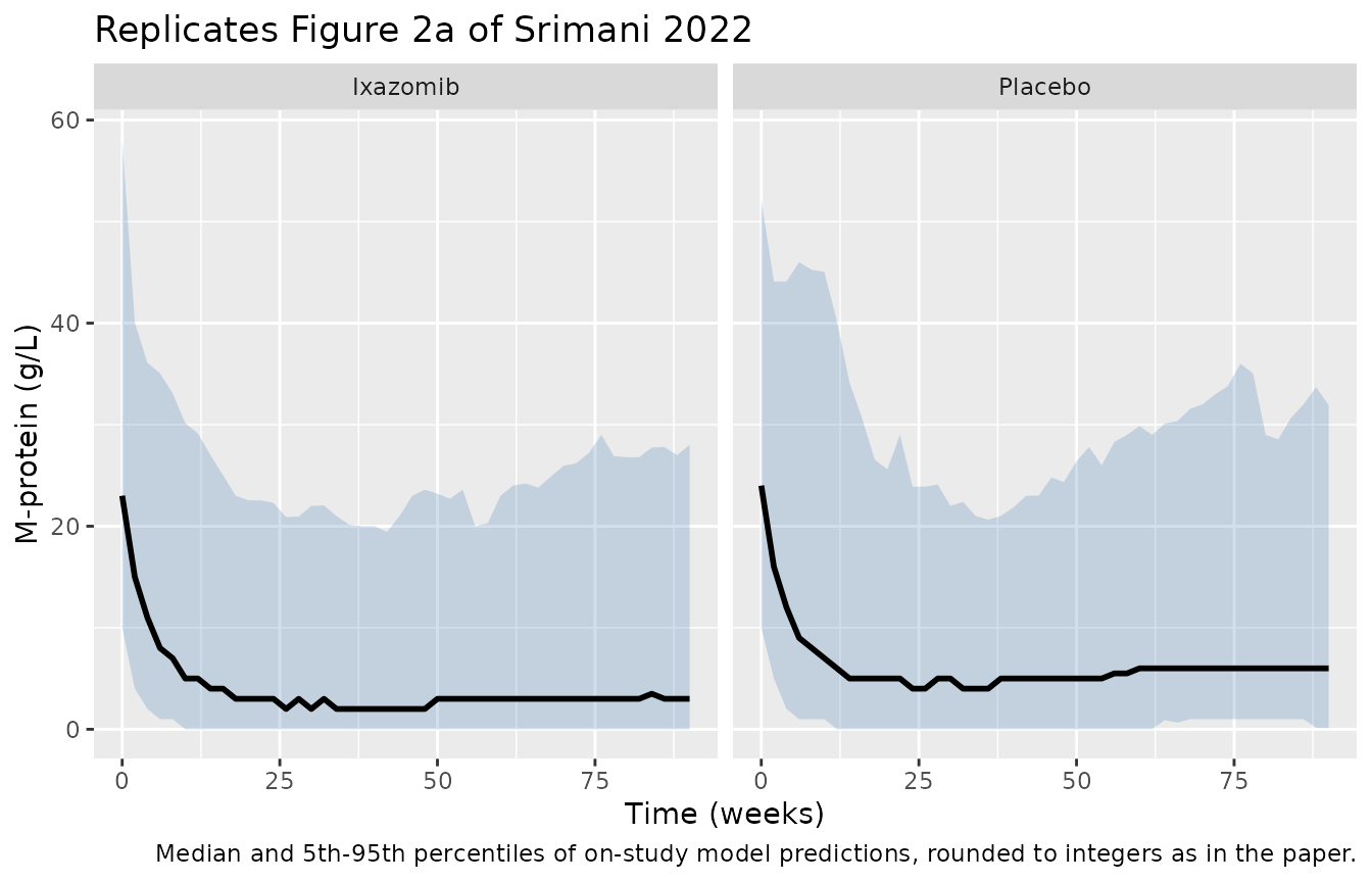
Figure 2a shows an observed median M-protein falling from the 23 g/L
baseline to about 3-5 g/L by week 20 and staying there, slightly lower
with ixazomib. The model reproduces the level and the arm ordering of
the median. Its upper tail is wider than the paper’s: the simulated 95th
percentile stays near 20-30 g/L, against a simulated 95% band of roughly
9-20 g/L in Figure 2a. The tail is set by the large inter-individual
variance of Yss (2.39, i.e. 155%; a patient at the 95th
percentile has a drug-free nadir above baseline), and the paper’s VPC
kept only the observation times of patients still on study, which this
virtual cohort can approximate only through the simulated dropout. The
95th percentile is therefore not gated.
# Typical (median) response depth: Yss = exp(-1.95) = 14.3% of a 23 g/L
# baseline is 3.3 g/L without ixazomib; a transcription error in kR, Yss, Imax
# or IC50 moves the week-40 median by several g/L.
stopifnot(
  all(mp_wk40$median >= 1 & mp_wk40$median <= 6),
  mp_wk40$median[mp_wk40$arm == "Ixazomib"] <= mp_wk40$median[mp_wk40$arm == "Placebo"]
)
Dropout, relapse and PFS (Figure 2b-d)
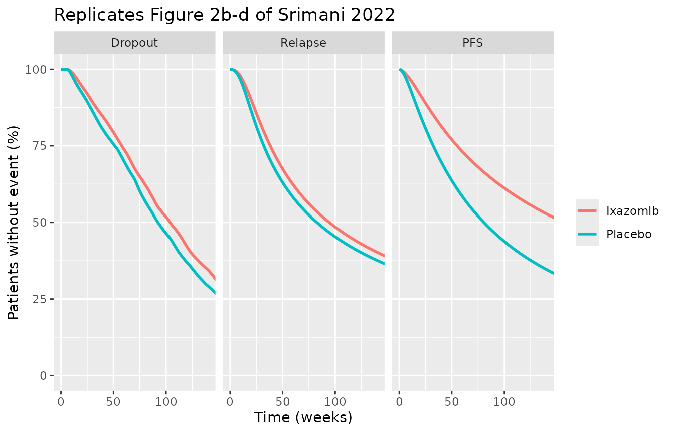
The curves below are the population-averaged survival from the cumulative hazards (the mean of the individual survival functions), which is what the Kaplan-Meier estimate of a large trial converges to.
surv_long <- pass2 |>
  group_by(arm, time) |>
  summarise(
    Dropout = mean(surv_drop), Relapse = mean(surv_relapse), PFS = mean(surv_pfs),
    .groups = "drop"
  ) |>
  pivot_longer(c(Dropout, Relapse, PFS), names_to = "endpoint", values_to = "surv") |>
  mutate(week = time / hr_per_week, endpoint = factor(endpoint, c("Dropout", "Relapse", "PFS")))
ggplot(surv_long, aes(week, 100 * surv, colour = arm)) +
  geom_line(linewidth = 1) +
  facet_wrap(~endpoint) +
  coord_cartesian(xlim = c(0, 140), ylim = c(0, 100)) +
  labs(
    x = "Time (weeks)", y = "Patients without event (%)", colour = NULL,
    title = "Replicates Figure 2b-d of Srimani 2022"
  )
median_week <- function(week, surv) {
  k <- which(surv < 0.5)
  if (length(k) == 0L) NA_real_ else week[k[1]]
}
pfs_tab <- surv_long |>
  filter(endpoint == "PFS") |>
  group_by(arm) |>
  summarise(sim_median_wk = median_week(week, surv), surv_120 = surv[week == 120]) |>
  mutate(
    obs_median_wk = ifelse(arm == "Ixazomib", 20.6, 14.7) * 365.25 / 12 / 7,
    pct_diff = 100 * (sim_median_wk / obs_median_wk - 1)
  )
pfs_tab |>
  dplyr::rename(
    "Arm" = arm, "Simulated median PFS (weeks)" = sim_median_wk,
    "Simulated PFS at 120 weeks" = surv_120, "Observed median PFS (weeks)" = obs_median_wk,
    "Difference (%)" = pct_diff
  ) |>
knitr::kable(digits = 2, caption = "Median PFS: model versus the trial (20.6 vs 14.7 months).")| Arm | Simulated median PFS (weeks) | Simulated PFS at 120 weeks | Observed median PFS (weeks) | Difference (%) |
|---|---|---|---|---|
| Ixazomib | 158 | 0.57 | 89.57 | 76.39 |
| Placebo | 82 | 0.39 | 63.92 | 28.29 |
The trial’s observed medians are a poor target here: Figure 2d shows the paper’s own simulations over-predicting ixazomib-arm PFS (the observed curve leaves the 95% band after week 100), and the Results call this “a slight overprediction of PFS”. The gate therefore compares the model with the paper’s simulated 95% bands, read off Figure 2b-d by the maintainers at weeks 80 and 120.
bands <- tribble(
  ~endpoint, ~arm, ~week, ~lo, ~hi,
  "Dropout", "Ixazomib", 80, 48, 63, "Dropout", "Ixazomib", 120, 22, 46,
  "Dropout", "Placebo", 80, 48, 62, "Dropout", "Placebo", 120, 22, 46,
  "Relapse", "Ixazomib", 80, 47, 58, "Relapse", "Ixazomib", 120, 33, 52,
  "Relapse", "Placebo", 80, 48, 60, "Relapse", "Placebo", 120, 33, 52,
  "PFS", "Ixazomib", 80, 60, 74, "PFS", "Ixazomib", 120, 45, 66,
  "PFS", "Placebo", 80, 50, 66, "PFS", "Placebo", 120, 38, 56
)
band_cmp <- bands |>
  left_join(surv_long |> mutate(endpoint = as.character(endpoint)) |> select(endpoint, arm, week, surv),
    by = c("endpoint", "arm", "week")
  ) |>
  mutate(sim = 100 * surv)
stopifnot(nrow(band_cmp) == 12, !anyNA(band_cmp$sim))
band_cmp |>
  select(endpoint, arm, week, sim, lo, hi) |>
  dplyr::rename(
    "Endpoint" = endpoint, "Arm" = arm, "Week" = week, "Simulated (%)" = sim,
    "Paper band low (%)" = lo, "Paper band high (%)" = hi
  ) |>
knitr::kable(digits = 1, caption = "Population-averaged survival against the simulated 95% bands of Figure 2b-d.")| Endpoint | Arm | Week | Simulated (%) | Paper band low (%) | Paper band high (%) |
|---|---|---|---|---|---|
| Dropout | Ixazomib | 80 | 62.4 | 48 | 63 |
| Dropout | Ixazomib | 120 | 42.0 | 22 | 46 |
| Dropout | Placebo | 80 | 57.1 | 48 | 62 |
| Dropout | Placebo | 120 | 36.9 | 22 | 46 |
| Relapse | Ixazomib | 80 | 54.4 | 47 | 58 |
| Relapse | Ixazomib | 120 | 43.9 | 33 | 52 |
| Relapse | Placebo | 80 | 50.8 | 48 | 60 |
| Relapse | Placebo | 120 | 41.0 | 33 | 52 |
| PFS | Ixazomib | 80 | 66.6 | 60 | 74 |
| PFS | Ixazomib | 120 | 56.7 | 45 | 66 |
| PFS | Placebo | 80 | 50.2 | 50 | 66 |
| PFS | Placebo | 120 | 38.7 | 38 | 56 |
# The digitised band edges carry about 2-3 points of reading error; 4 points
# of slack keeps the gate from tripping on that while a wrong hazard
# parameter (time unit, sign, centring) moves these values by 10-40 points.
stopifnot(all(band_cmp$sim > band_cmp$lo - 4 & band_cmp$sim < band_cmp$hi + 4))
pfs_ratio <- pfs_tab$sim_median_wk[pfs_tab$arm == "Ixazomib"] /
  pfs_tab$sim_median_wk[pfs_tab$arm == "Placebo"]
# Ixazomib must lengthen PFS: a weekly-AUC coefficient read per ug*h/mL would
# remove the drug effect and give a ratio near 1.
stopifnot(pfs_ratio > 1.3)
Dropout, relapse and PFS all fall inside the paper’s simulated bands. The simulated median PFS is about 30% longer than observed on placebo and longer still with ixazomib, the same over-prediction the paper’s Figure 2d shows.
Platelet count (Figure 4 and Supplementary Figure S14)
mod_plt <- readModelDb("Srimani_2022_ixazomib_platelets")
plt_times <- seq(0, 24 * 7 * 24, by = 24 * 3.5)
plt_ev <- build_events(cohort, plt_times, "circ", ncycle = 6, len_doses = TRUE)
eta_plt <- draw_etas(mod_plt, nrow(cohort), seed = 201)
#> ℹ parameter labels from comments will be replaced by 'label()'
#> Warning: some etas defaulted to non-mu referenced, possible parsing error: etabl
#> as a work-around try putting the mu-referenced expression on a simple line
plt_sim <- solve_ind(mod_plt, plt_ev, eta_plt) |>
  left_join(cohort |> select(id, arm), by = "id") |>
  mutate(week = time / hr_per_week)
#> ℹ parameter labels from comments will be replaced by 'label()'
#> Warning: some etas defaulted to non-mu referenced, possible parsing error: etabl
#> as a work-around try putting the mu-referenced expression on a simple line
#> Warning: some etas defaulted to non-mu referenced, possible parsing error: etabl
#> as a work-around try putting the mu-referenced expression on a simple line
#> Warning: multi-subject simulation without without 'omega'
plt_sum <- plt_sim |>
  group_by(arm, week) |>
  summarise(median = median(PLT), p10 = quantile(PLT, 0.1), p90 = quantile(PLT, 0.9), .groups = "drop")
ggplot(plt_sum, aes(week)) +
  geom_ribbon(aes(ymin = p10, ymax = p90), fill = "steelblue", alpha = 0.25) +
  geom_line(aes(y = median), linewidth = 1) +
  geom_hline(yintercept = c(50, 75), linetype = "dashed") +
  facet_wrap(~arm) +
  labs(
    x = "Time (weeks)", y = expression("Platelet count (" * 10^9 * "/L)"),
    title = "Replicates Figure 4 and Supplementary Figure S14 of Srimani 2022 (first 6 cycles)",
    caption = "Model-predicted median and 10th-90th percentiles without residual error."
  )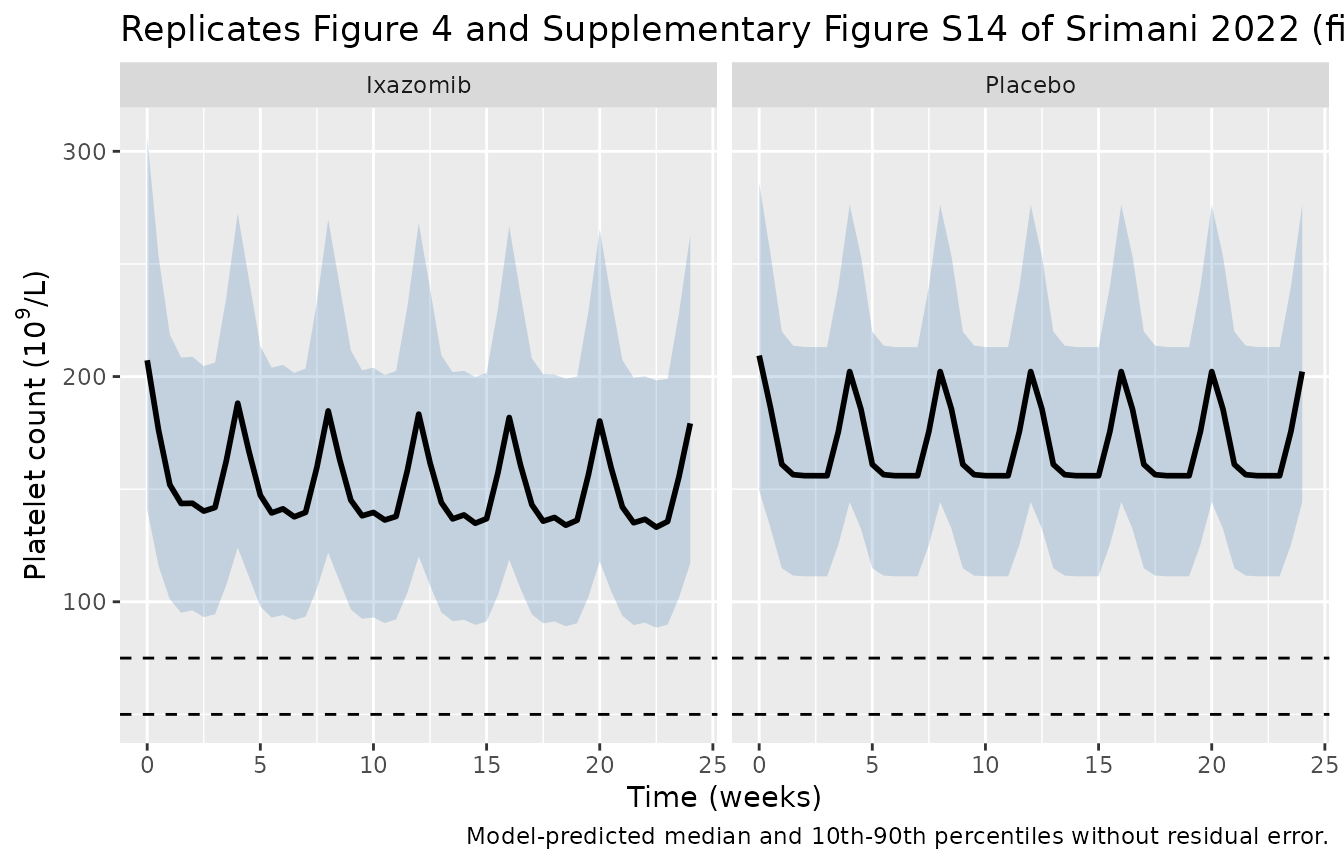
In the placebo arm of Supplementary Figure S14 the observed median falls from about 195 to about 150-165 x 10^9/L in weeks 2-3 of each cycle and recovers to about 200 in the rest week; Figure 4 shows the same pattern with ixazomib, a few percent lower. The typical-value check below pins that cycle.
typ_ev <- data.frame(id = 1L, time = c(len_dose_times(1), seq(0, 28 * 24, by = 12)))
typ_ev$amt <- c(rep(25, 21), rep(0, nrow(typ_ev) - 21))
typ_ev$evid <- c(rep(1L, 21), rep(0L, nrow(typ_ev) - 21))
typ_ev$cmt <- c(rep("depot_kpd", 21), rep("circ", nrow(typ_ev) - 21))
typ_ev$BSA <- 1.87
typ_ev$PLT_BASE <- 197
typ <- as.data.frame(rxode2::rxSolve(rxode2::zeroRe(mod_plt), typ_ev[order(typ_ev$time, -typ_ev$evid), ],
  returnType = "data.frame"
))
#> ℹ parameter labels from comments will be replaced by 'label()'
#> Warning: some etas defaulted to non-mu referenced, possible parsing error: etabl
#> as a work-around try putting the mu-referenced expression on a simple line
#> Warning: some etas defaulted to non-mu referenced, possible parsing error: etabl
#> as a work-around try putting the mu-referenced expression on a simple line
#> ℹ omega/sigma items treated as zero: 'etalcl', 'etalfdepot', 'etalvp2', 'etabl'
typ_nadir <- min(typ$PLT)
typ_day28 <- typ$PLT[typ$time == 28 * 24]
c(baseline = typ$PLT[1], nadir = typ_nadir, day28 = typ_day28)
#> baseline    nadir    day28
#> 203.0000 151.2396 196.1002
# Deterministic typical placebo cycle: 203 -> ~151 -> ~196 x 10^9/L. Driving
# the LenDex effect by the K-PD amount instead of its rate gives a nadir near
# 26, and a slope transcribed per week instead of per hour gives ~0.
stopifnot(typ_nadir > 140, typ_nadir < 165, typ_day28 > 185)
Diarrhea and rash (Discrete-time Markov models)
Transition matrices without drug, time or covariate effects
With no ixazomib, no explicit time effect and the reference covariates, the model’s transition probabilities must equal the matrices printed in Appendix S1 (Supplementary Equation S3 for diarrhea, IMiD-exposed; Supplementary Equation 14 for rash, non-Asian). The printed matrices list the destination grade by row (3, 2, 1, 0) and the current grade by column.
mod_dia <- readModelDb("Srimani_2022_ixazomib_diarrhea")
mod_rash <- readModelDb("Srimani_2022_ixazomib_rash")
base_ev <- data.frame(id = 1L, time = 1000, amt = 0, evid = 0L, cmt = "central", BSA = 1.87, PRIOR_IMMUNOMODULATORY_DRUG = 1, RACE_ASIAN = 0)
pnames <- paste0("p", rep(0:3, each = 4), rep(0:3, 4))
to_matrix <- function(s) matrix(unlist(s[1, pnames]), 4, 4, byrow = TRUE)
dia_base <- to_matrix(rxode2::rxSolve(rxode2::zeroRe(mod_dia), base_ev,
  params = c(lemax_time_g10 = -Inf, e_week1_g01 = 0), returnType = "data.frame"
))
#> ℹ parameter labels from comments will be replaced by 'label()'
#> Warning: No sigma parameters in the model
#> [====|====|====|====|====|====|====|====|====|====] 0:00:00
#> ℹ omega/sigma items treated as zero: 'etalcl', 'etalfdepot', 'etalvp2', 'etab01', 'etab11', 'etab21', 'etab31'
rash_base <- to_matrix(rxode2::rxSolve(rxode2::zeroRe(mod_rash), base_ev,
  params = c(lemax_time_g10 = -Inf, e_transient_g0 = 0), returnType = "data.frame"
))
#> ℹ parameter labels from comments will be replaced by 'label()'
#> Warning: No sigma parameters in the model
#> [====|====|====|====|====|====|====|====|====|====] 0:00:00
#> ℹ omega/sigma items treated as zero: 'etalcl', 'etalfdepot', 'etalvp2', 'etab01', 'etab11', 'etab21'
# Supplementary Equations S3 and 14, rows = destination grade 3, 2, 1, 0;
# columns = current grade 3, 2, 1, 0.
s3 <- matrix(c(
  0.966, 0.000637, 0.000236, 0.000215,
  0.00515, 0.856, 0.00108, 0.00126,
  0.00308, 0.0171, 0.662, 0.00357,
  0.0258, 0.126, 0.337, 0.995
), 4, 4, byrow = TRUE)
s14 <- matrix(c(
  0.843, 0.00260, 0.00128, 0.0000361,
  0.0143, 0.799, 0.00103, 0.000134,
  0.00714, 0.0124, 0.597, 0.000459,
  0.136, 0.186, 0.401, 0.999
), 4, 4, byrow = TRUE)
# Reorder the published matrices to current grade (row) 0-3 by destination
# grade (column) 0-3.
from_pub <- function(m) t(m)[4:1, 4:1]
round(dia_base, 5)
#>         [,1]    [,2]    [,3]    [,4]
#> [1,] 0.99493 0.00359 0.00126 0.00022
#> [2,] 0.33693 0.66176 0.00107 0.00023
#> [3,] 0.12565 0.01701 0.85668 0.00066
#> [4,] 0.02583 0.00310 0.00513 0.96594
round(rash_base, 5)
#>         [,1]    [,2]    [,3]    [,4]
#> [1,] 0.99937 0.00046 0.00013 0.00004
#> [2,] 0.40083 0.59690 0.00101 0.00126
#> [3,] 0.18543 0.01246 0.79942 0.00269
#> [4,] 0.13587 0.00715 0.01427 0.84270
rel_err_dia <- abs(dia_base / from_pub(s3) - 1)
rel_err_rash <- abs(rash_base / from_pub(s14) - 1)
# Same parameters, same formula: only the 3-significant-figure rounding of
# the printed matrices and of the tables separates the two sides. The largest
# gaps are both grade-2-to-3 cells (diarrhea 4%, rash 3%), where the rounded
# B23 (2.21, 1.99) enters through exp(). A mis-transcribed B parameter moves
# its cells by tens of percent.
c(diarrhea = max(rel_err_dia), rash = max(rel_err_rash))
#>   diarrhea       rash
#> 0.03640411 0.03412754
stopifnot(max(rel_err_dia) < 0.05, max(rel_err_rash) < 0.05)
Transitions out of grade 0 versus weekly AUC (Supplementary Figures S10 and S12)
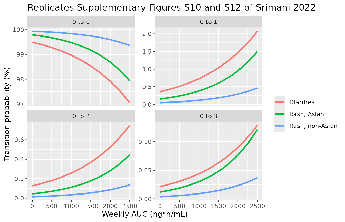
The ixazomib effect is linear in the weekly AUC on the logits out of
grade 0. Shifting b01 by slp_aucwk_g0 * AUC
for a drug-free patient traces the curves of Supplementary Figures S10
and S12.
auc_grid <- seq(0, 2500, by = 250)
grid_ev <- data.frame(id = seq_along(auc_grid), time = 1000, amt = 0, evid = 0L, cmt = "central", BSA = 1.87, PRIOR_IMMUNOMODULATORY_DRUG = 1, RACE_ASIAN = 0)
curve_one <- function(mod, b01, slp, label, asian = 0) {
  ev <- grid_ev
  ev$RACE_ASIAN <- asian
  p <- data.frame(id = ev$id, b01 = b01 + slp * auc_grid, lemax_time_g10 = -Inf)
  if ("e_week1_g01" %in% rxode2::rxode(mod)$iniDf$name) p$e_week1_g01 <- 0
  if ("e_transient_g0" %in% rxode2::rxode(mod)$iniDf$name) p$e_transient_g0 <- 0
  s <- as.data.frame(rxode2::rxSolve(rxode2::zeroRe(mod), ev, params = p, returnType = "data.frame"))
  tibble(model = label, AUC = auc_grid, `0 to 0` = s$p00, `0 to 1` = s$p01, `0 to 2` = s$p02, `0 to 3` = s$p03)
}
curves <- bind_rows(
  curve_one(mod_dia, -5.28, 0.000715, "Diarrhea"),
  curve_one(mod_rash, -7.37, 0.000929, "Rash, non-Asian"),
  curve_one(mod_rash, -7.37, 0.000929, "Rash, Asian", asian = 1)
) |>
  pivot_longer(-c(model, AUC), names_to = "transition", values_to = "p")
#> ℹ parameter labels from comments will be replaced by 'label()'
#> ℹ parameter labels from comments will be replaced by 'label()'
#> ℹ parameter labels from comments will be replaced by 'label()'
#> Warning: No sigma parameters in the model
#> ℹ omega/sigma items treated as zero: 'etalcl', 'etalfdepot', 'etalvp2', 'etab01', 'etab11', 'etab21', 'etab31'
#> ℹ parameter labels from comments will be replaced by 'label()'
#> ℹ parameter labels from comments will be replaced by 'label()'
#> ℹ parameter labels from comments will be replaced by 'label()'
#> Warning: No sigma parameters in the model
#> ℹ omega/sigma items treated as zero: 'etalcl', 'etalfdepot', 'etalvp2', 'etab01', 'etab11', 'etab21'
#> ℹ parameter labels from comments will be replaced by 'label()'
#> ℹ parameter labels from comments will be replaced by 'label()'
#> ℹ parameter labels from comments will be replaced by 'label()'
#> Warning: No sigma parameters in the model
#> ℹ omega/sigma items treated as zero: 'etalcl', 'etalfdepot', 'etalvp2', 'etab01', 'etab11', 'etab21'
ggplot(curves, aes(AUC, 100 * p, colour = model)) +
  geom_line(linewidth = 1) +
  facet_wrap(~transition, scales = "free_y") +
  labs(
    x = "Weekly AUC (ng*h/mL)", y = "Transition probability (%)", colour = NULL,
    title = "Replicates Supplementary Figures S10 and S12 of Srimani 2022"
  )
end_vals <- curves |>
  filter(AUC == 2500, transition != "0 to 0") |>
  pivot_wider(names_from = transition, values_from = p)
knitr::kable(end_vals |> mutate(across(-model, ~ 100 * .x)), digits = 3, caption = "Transition probabilities (%) at a weekly AUC of 2500 ng*h/mL.")| model | AUC | 0 to 1 | 0 to 2 | 0 to 3 |
|---|---|---|---|---|
| Diarrhea | 250000 | 2.075 | 0.749 | 0.128 |
| Rash, non-Asian | 250000 | 0.465 | 0.136 | 0.037 |
| Rash, Asian | 250000 | 1.501 | 0.446 | 0.121 |
# Read off the figures by the maintainers at AUC = 2500: diarrhea 0 to 1
# ~2.05%, 0 to 2 ~0.73%; rash Asian 0 to 1 ~1.5%, non-Asian ~0.45%.
stopifnot(
  abs(100 * end_vals$`0 to 1`[end_vals$model == "Diarrhea"] - 2.05) < 0.2,
  abs(100 * end_vals$`0 to 2`[end_vals$model == "Diarrhea"] - 0.73) < 0.1,
  abs(100 * end_vals$`0 to 1`[end_vals$model == "Rash, Asian"] - 1.5) < 0.15,
  abs(100 * end_vals$`0 to 1`[end_vals$model == "Rash, non-Asian"] - 0.45) < 0.08
)
One-year grade prevalence for typical patients
The paper reports model-predicted prevalence after one year: for diarrhea, grade 3 in 1.2% of ixazomib-treated IMiD-exposed patients, 0.1% of IMiD-naive patients, and 0.5% versus 0.1% on placebo (Results); for rash, grade 0/1/2/3 in 97.3/2.4/0.2/0.1% of non-Asian and 91.5/7.5/0.7/0.3% of Asian ixazomib-treated patients, and grade 0 in 99.1% versus 97.3% of non-Asian and Asian placebo patients (Supplement 2.2.2). The supplement calls the one-year values steady state, and they are reproduced when ixazomib is given every week without the rest week, so that the weekly AUC settles at F x Dose / CL = 1247 ng*h/mL; on the trial schedule (3 of 4 weeks) the ixazomib-arm grade 1-3 values come out about a quarter lower. The typical-value Markov chains below use the weekly transition probabilities of a typical patient on that continuous schedule.
week_times <- seq(1, 52) * hr_per_week
typ_cohort <- tidyr::expand_grid(arm = c("Ixazomib", "Placebo"), PRIOR_IMMUNOMODULATORY_DRUG = c(1, 0), RACE_ASIAN = c(0, 1)) |>
  mutate(id = row_number(), BSA = 1.87, MCPROT = 23, TUM_CYTOGENETIC_HIGH_RISK = 0, PLT_BASE = 197)
# 4 mg every week (no rest week) for 53 weeks.
typ_ev <- bind_rows(
  typ_cohort |> filter(arm == "Ixazomib") |> select(id) |>
    tidyr::crossing(time = seq(0, 52) * hr_per_week) |> mutate(amt = 4, evid = 1L, cmt = "depot"),
  typ_cohort |> select(id) |> tidyr::crossing(time = week_times) |> mutate(amt = 0, evid = 0L, cmt = "central")
) |>
  left_join(typ_cohort, by = "id") |>
  arrange(id, time, desc(evid))
one_year <- function(mod, label) {
  s <- as.data.frame(rxode2::rxSolve(rxode2::zeroRe(mod), typ_ev, atol = 1e-6, rtol = 1e-6, returnType = "data.frame"))
  s |>
    group_by(id) |>
    group_modify(~ {
      x <- markov_expected(.x)
      tibble(G0 = x[52, 1], G1 = x[52, 2], G2 = x[52, 3], G3 = x[52, 4])
    }) |>
    ungroup() |>
    left_join(typ_cohort |> select(id, arm, PRIOR_IMMUNOMODULATORY_DRUG, RACE_ASIAN), by = "id") |>
    mutate(model = label)
}
dia_1y <- one_year(mod_dia, "Diarrhea") |> filter(RACE_ASIAN == 0)
#> ℹ parameter labels from comments will be replaced by 'label()'
#> Warning: No sigma parameters in the model
#> ℹ omega/sigma items treated as zero: 'etalcl', 'etalfdepot', 'etalvp2', 'etab01', 'etab11', 'etab21', 'etab31'
rash_1y <- one_year(mod_rash, "Rash") |> filter(PRIOR_IMMUNOMODULATORY_DRUG == 1)
#> ℹ parameter labels from comments will be replaced by 'label()'
#> Warning: No sigma parameters in the model
#> ℹ omega/sigma items treated as zero: 'etalcl', 'etalfdepot', 'etalvp2', 'etab01', 'etab11', 'etab21'

dia_tab <- dia_1y |>
  transmute(arm, IMiD = ifelse(PRIOR_IMMUNOMODULATORY_DRUG == 1, "exposed", "naive"), sim_G3 = 100 * G3) |>
  mutate(paper_G3 = c(1.2, 0.1, 0.5, 0.1)[match(paste(arm, IMiD), c("Ixazomib exposed", "Ixazomib naive", "Placebo exposed", "Placebo naive"))])
dia_tab |>
  dplyr::rename("Arm" = arm, "Prior IMiD" = IMiD, "Simulated grade 3 (%)" = sim_G3, "Paper grade 3 (%)" = paper_G3) |>
knitr::kable(digits = 2, caption = "Diarrhea grade 3 prevalence after one year.")| Arm | Prior IMiD | Simulated grade 3 (%) | Paper grade 3 (%) |
|---|---|---|---|
| Ixazomib | exposed | 1.22 | 1.2 |
| Ixazomib | naive | 0.13 | 0.1 |
| Placebo | exposed | 0.54 | 0.5 |
| Placebo | naive | 0.06 | 0.1 |
rash_tab <- rash_1y |>
  transmute(arm, race = ifelse(RACE_ASIAN == 1, "Asian", "non-Asian"), G0 = 100 * G0, G1 = 100 * G1, G2 = 100 * G2, G3 = 100 * G3)
rash_paper <- tibble(
  arm = c("Ixazomib", "Ixazomib", "Placebo", "Placebo"), race = c("non-Asian", "Asian", "non-Asian", "Asian"),
  paper_G0 = c(97.3, 91.5, 99.1, 97.3), paper_G1 = c(2.4, 7.5, NA, NA)
)
rash_cmp <- left_join(rash_tab, rash_paper, by = c("arm", "race"))
rash_cmp |>
  dplyr::rename("Arm" = arm, "Race" = race, "Sim G0 (%)" = G0, "Sim G1 (%)" = G1, "Sim G2 (%)" = G2, "Sim G3 (%)" = G3, "Paper G0 (%)" = paper_G0, "Paper G1 (%)" = paper_G1) |>
knitr::kable(digits = 2, caption = "Rash grade prevalence after one year.")| Arm | Race | Sim G0 (%) | Sim G1 (%) | Sim G2 (%) | Sim G3 (%) | Paper G0 (%) | Paper G1 (%) |
|---|---|---|---|---|---|---|---|
| Ixazomib | non-Asian | 97.33 | 2.35 | 0.23 | 0.09 | 97.3 | 2.4 |
| Ixazomib | Asian | 91.77 | 7.23 | 0.70 | 0.29 | 91.5 | 7.5 |
| Placebo | non-Asian | 99.14 | 0.76 | 0.07 | 0.03 | 99.1 | NA |
| Placebo | Asian | 97.24 | 2.43 | 0.23 | 0.10 | 97.3 | NA |
# Deterministic typical-value chains; the gaps left are the rounding of the
# printed percentages. With the slow time effect on the grade 0 -> 1 logit
# instead of on recovery from grade 1, the AUC-free placebo rash values are
# 98.9% / 96.4% grade 0 (paper 99.1% / 97.3%) and this gate fails.
stopifnot(
  all(abs(dia_tab$sim_G3 - dia_tab$paper_G3) < 0.15),
  all(abs(rash_cmp$G0 - rash_cmp$paper_G0) < 0.5),
  all(abs(rash_cmp$G1 - rash_cmp$paper_G1) < 0.5, na.rm = TRUE)
)
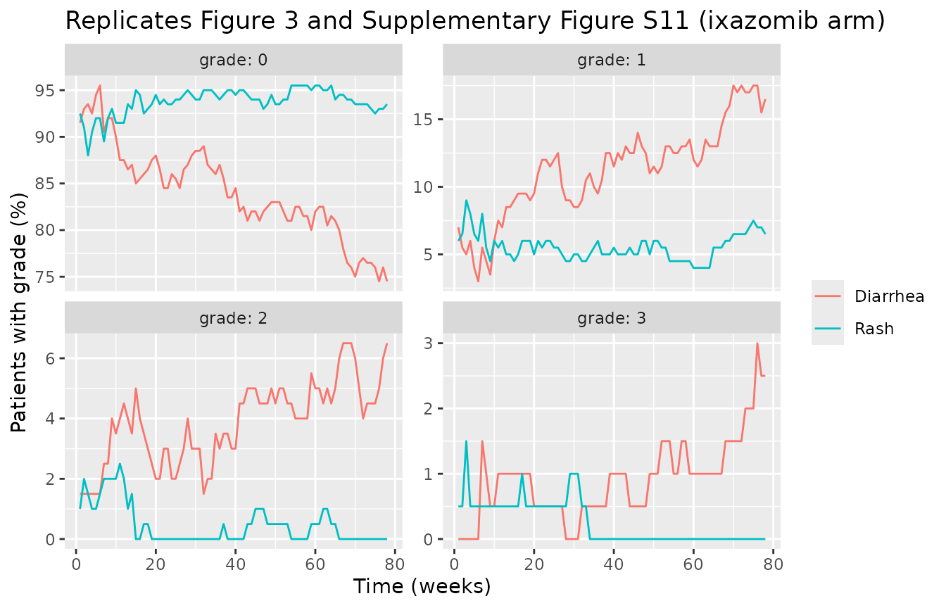
Diarrhea and rash prevalence over time (Figure 3 and Supplementary Figure S11)
Individual grade sequences are drawn week by week from each simulated patient’s transition probabilities, with the per-grade random intercepts.
ae_weeks <- seq(1, 78)
ae_ev <- build_events(cohort, ae_weeks * hr_per_week, "central", ncycle = 20)
ae_prev <- function(mod, label, seed) {
  etas <- draw_etas(mod, nrow(cohort), seed = seed)
  s <- solve_ind(mod, ae_ev, etas) |> arrange(id, time)
  set.seed(seed + 1)
  s$grade <- markov_walk(s, stats::runif(nrow(s)))
  s |>
    left_join(cohort |> select(id, arm), by = "id") |>
    mutate(week = time / hr_per_week) |>
    count(arm, week, grade) |>
    group_by(arm, week) |>
    mutate(pct = 100 * n / sum(n)) |>
    ungroup() |>
    tidyr::complete(arm, week, grade = 0:3, fill = list(n = 0, pct = 0)) |>
    mutate(model = label)
}
ae <- bind_rows(ae_prev(mod_dia, "Diarrhea", 301), ae_prev(mod_rash, "Rash", 401))
#> ℹ parameter labels from comments will be replaced by 'label()'
#> ℹ parameter labels from comments will be replaced by 'label()'
#> Warning: No sigma parameters in the model
#> ℹ parameter labels from comments will be replaced by 'label()'
#> ℹ parameter labels from comments will be replaced by 'label()'
#> Warning: No sigma parameters in the model
ggplot(ae |> filter(arm == "Ixazomib"), aes(week, pct, colour = model)) +
  geom_line() +
  facet_wrap(~grade, scales = "free_y", labeller = label_both) +
  labs(
    x = "Time (weeks)", y = "Patients with grade (%)", colour = NULL,
    title = "Replicates Figure 3 and Supplementary Figure S11 (ixazomib arm)"
  )
ae_pts <- ae |>
  filter(arm == "Ixazomib", week %in% c(4, 40, 76)) |>
  select(model, week, grade, pct) |>
  pivot_wider(names_from = grade, values_from = pct, names_prefix = "grade ")
knitr::kable(ae_pts, digits = 1, caption = "Simulated prevalence (%) in the ixazomib arm.")| model | week | grade 0 | grade 1 | grade 2 | grade 3 |
|---|---|---|---|---|---|
| Diarrhea | 4 | 92.5 | 6.0 | 1.5 | 0.0 |
| Diarrhea | 40 | 84.5 | 11.5 | 3.0 | 1.0 |
| Diarrhea | 76 | 74.5 | 17.5 | 5.0 | 3.0 |
| Rash | 4 | 90.5 | 8.0 | 1.0 | 0.5 |
| Rash | 40 | 94.5 | 5.5 | 0.0 | 0.0 |
| Rash | 76 | 93.0 | 7.0 | 0.0 | 0.0 |
Figure 3 shows observed grade-0 diarrhea in the ixazomib arm falling from about 90% to 80% over 75 weeks while grade 1 rises from about 5% to 13%; Supplementary Figure S11 shows rash concentrated in the first weeks (grade 0 about 87% at week 4, about 95% from week 40). The simulated sequences follow both shapes.
g <- function(model, week, grade) ae_pts[[paste("grade", grade)]][ae_pts$model == model & ae_pts$week == week]
# 200 patients per arm drawn with a fixed R seed: the margins admit the
# Monte-Carlo spread of a 200-patient prevalence (a few percentage points).
stopifnot(
  g("Diarrhea", 76, 0) < g("Diarrhea", 4, 0),
  g("Diarrhea", 76, 0) > 65, g("Diarrhea", 76, 0) < 92,
  g("Rash", 4, 0) < g("Rash", 40, 0),
  g("Rash", 40, 0) > 88
)
Assumptions and deviations
-
Weekly AUC. The paper integrates the PK model to a
weekly AUC without stating the window. The models use the AUC over the
168 h ending at the evaluation time, computed with
delay(). This needs a dense solver, and an occasional patient fails at the default tolerances;atol = rtol = 1e-6avoids it. -
Weekly-AUC units. Table 2 labels the PFS
coefficient
ml/(ug.h), but its “untransformed” value exp(-0.00108) = 0.999 uses the estimate as printed, and Table 3 converts the diarrhea slope from 0.000715 to 0.715 per ugh/mL while Supplementary Figures S10 and S12 plot AUC in ngh/mL. All AUC coefficients are therefore read per ng*h/mL. On a per-ug reading the PFS model would carry no ixazomib effect, against the trial’s PFS difference. -
Nadir time.
T_MPROTEIN_NADIRis a covariate, because the paper derived it from each patient’s observed profile. The vignette draws it from the relapse hazard. The 4.71% of patients without an estimable nadir (p_tnadir0) were excluded from the paper’s PK/PD fit; the vignette does not simulate them separately. -
Relapse parameters. Table 2 prints the same
estimate, 0.0509, for
alpha_IXAandalpha_kR,0, with different standard errors and confidence intervals. Both are used as printed. The relapse multiplierlambda0(exp(-1.23) = 0.292) multiplies a log-logistic hazard and is dimensionless on the model’s hour time base, although Table 2 converts it to 49.0/week. -
Platelet loss rate. The paper gives no separate
kout. Because the system is normalised to baseline with productionkIn, the circulating loss rate equalskIn, and the precursor states start atkIn / kprp. -
Lenalidomide K-PD driver. “Len conc.” is read as
the K-PD effect rate
kLEN * A(mg/h; Jacqmin 2007). Driving the effect by the amountAitself drops the placebo platelet count to about 13% of baseline within a cycle, against the 20-25% dip of Supplementary Figure S14. Lenalidomide doses are given as 25 mg; patients with reduced creatinine clearance received 10 mg. -
Markov time effects. The functional form and target
of the slow time effect (
P1|0T,K1|0T) are not printed, and the main text describes it as a “slow transition from grade 0 to grade 1”. Appendix S1 writesp_i|jfor the move from grade i to grade j, which makesP1|0the grade-1-to-0 recovery andP0|1the grade-0-to-1 onset (the diarrheaP0|1I, “rapid diarrhea onset in week 1”). The models therefore addexp(P1|0T) * (1 - exp(-K * t))to the grade >= 1 logit from grade 1, which slows recovery and raises grade 1 prevalence over time, the effect both models are said to describe. This placement and form reproduce every one-year prevalence the paper prints; putting the same term on the grade-0-to-1 logit misses the AUC-free placebo rash values and roughly doubles the late grade-1 diarrhea of Figure 3. The diarrheaP0|1Iterm is added to the grade-0-to-1 logit during the first 168 h. The rash transientETIME * exp(-KTIME * t)shifts every logit out of grade 0, which gives the early grade 2-3 rash of Supplementary Figure S11. - Typical exposure behind the one-year values. The paper’s one-year (“steady state”) predictions are reproduced with uninterrupted weekly dosing (weekly AUC 1247 ng*h/mL), not with the 3-of-4-week trial schedule.
-
Covariate reference groups. The printed diarrhea
matrix is the IMiD-exposed one, so the IMiD shift applies to naive
patients (
1 - PRIOR_IMMUNOMODULATORY_DRUG); the M-proteinYsseffect is coded the same way. - Likelihood. The Markov models emit transition probabilities only; their categorical likelihood conditioned on the previous grade cannot be written as an nlmixr2 observation, so these files are for simulation.
- M-protein upper tail. The simulated on-study 95th percentile of M-protein is about 1.5 times the paper’s simulated band (see the Figure 2a section); the median is reproduced.
- Virtual cohort. BSA, baseline M-protein and baseline platelet count are drawn from log-normal or normal distributions matched to the reported medians; the paper reports no BSA distribution.