Extended-release levetiracetam in epileptic dogs (Munana 2018)
Source:vignettes/articles/Munana_2018_levetiracetam_dog.Rmd
Munana_2018_levetiracetam_dog.RmdModel and source
- Citation: Munana KR, Otamendi AJ, Nettifee JA, Papich MG. Population pharmacokinetics of extended-release levetiracetam in epileptic dogs when administered alone, with phenobarbital or zonisamide. J Vet Intern Med. 2018;32(5):1677-1683. doi:10.1111/jvim.15298. Structural and random-effect forms taken from the Supporting Information (JVIM-32-1677-s001.pdf, Equations 2-4); parameter values from Table 1.
- Description: Veterinary (dog). One-compartment population PK model with first-order absorption and first-order elimination for extended-release levetiracetam (LEV-XR) in client-owned dogs with idiopathic epilepsy, sampled at steady state on their established q12h maintenance regimen. Parameterised in rate-constant form (k01, k10, V/F) per kg body weight, as published. Absorption is slower than elimination, so the terminal slope is absorption-limited (flip-flop) and the apparent 5 h terminal half-life is the absorption half-life. Concomitant phenobarbital raises the apparent volume of distribution V/F about 2.6-fold, lowering Cmax and AUC; concomitant zonisamide has no effect (Munana 2018)
- Article: https://doi.org/10.1111/jvim.15298 (open access)
- Supporting Information:
JVIM-32-1677-s001.pdf, reachable from the article landing page and from the EuropePMC record PMC6189379
This is a veterinary (dog) model. Munana and colleagues sampled 18 client-owned dogs with idiopathic epilepsy who were already on stable q12h maintenance therapy with extended-release levetiracetam (LEV-XR), either alone or alongside phenobarbital or zonisamide, and fitted a one-compartment model with first-order absorption and first-order elimination to the resulting sparse steady-state data.
Two features of the model are worth flagging before any simulation:
-
It is parameterised by rate constants, not by
clearance. The source fits
k01,k10andV/Fwith an independent exponential random effect on each (Supporting Information Equation 2). Recasting it ascl+vcwould require a correlated eta block that the authors did not fit, so the model file keepslka/lkel/lvc. -
It is flip-flop.
k01(0.138 1/h) is well belowk10(0.505 1/h), so absorption, not elimination, is rate-limiting and the terminal slope of the profile reports the absorption half-life of about 5 h. The paper is explicit about this (“this value can be misinterpreted because of the ‘flip-flop’ phenomenon”), and the NCA section below verifies it.
Everything is published per kg body weight, and the source normalised every observed concentration to the study mean dose of 29.4 mg/kg before fitting, so doses in this vignette are given in mg/kg and concentrations come out in ug/mL.
Population
Eighteen client-owned dogs with a presumptive diagnosis of idiopathic epilepsy (at minimum International Veterinary Epilepsy Task Force tier 1 confidence) were enrolled six per group: LEV-XR alone (L), LEV-XR plus phenobarbital (LP), and LEV-XR plus zonisamide (LZ). One LZ dog receiving more than 200 mg/kg of LEV-XR was excluded before the population fit, so 17 dogs contributed. Breeds were mixed breed (6), Labrador retriever (3), Australian shepherd (2) and one each of Basset hound, Golden retriever, Pembroke Welsh corgi, Vizsla, Curly-coated retriever and English springer spaniel. There were 11 spayed females and 6 neutered males, median body weight 25.7 kg (range 7.8-45.5), age 3-12 years (median 6), and median epilepsy duration 1 year (Results, “Dog demographics”).
Every dog had to be at steady state on all of its antiepileptic drugs, with no dose change for at least five half-lives. The LP group received a mean phenobarbital dose of 2.86 mg/kg q12h (mean trough serum concentration 28.48 ug/mL) and the LZ group a mean zonisamide dose of 7.82 mg/kg q12h (mean trough 55.09 ug/mL). LEV-XR dose per dog was 500 mg in 8 dogs, 750 mg in 7, 1000 mg in 1 and 1500 mg in 1, giving group mean doses of 31.86, 30.91 and 23.52 mg/kg in the L, LP and LZ groups and a study mean of 29.4 mg/kg (Results, “AED administration”). Five samples were drawn per dog, at 0 (pre-dose trough), 2, 4, 8 and 12 h after the morning dose, which was given with food.
The same information is available programmatically from the model’s
population metadata:
pop <- rxode2::rxode(readModelDb("Munana_2018_levetiracetam_dog"))$population
#> ℹ parameter labels from comments will be replaced by 'label()'
str(pop, max.level = 1)
#> List of 15
#>  $ species       : chr "dog (client-owned; mixed breed n = 6, Labrador retriever n = 3, Australian shepherd n = 2, and one each of Bass"| __truncated__
#>  $ n_subjects    : int 17
#>  $ n_enrolled    : int 18
#>  $ n_studies     : int 1
#>  $ n_observations: int 85
#>  $ age_range     : chr "3-12 years"
#>  $ age_median    : chr "6 years"
#>  $ weight_range  : chr "7.8-45.5 kg"
#>  $ weight_median : chr "25.7 kg"
#>  $ sex_female_pct: num 64.7
#>  $ disease_state : chr "idiopathic epilepsy, at least International Veterinary Epilepsy Task Force tier 1 confidence, median duration 1 year"
#>  $ dose_range    : chr "500, 750, 1000 or 1500 mg LEV-XR PO q12h per dog (group means 31.86, 30.91 and 23.52 mg/kg in the L, LP and LZ "| __truncated__
#>  $ co_medication : chr "6 dogs LEV-XR alone (L), 6 LEV-XR + phenobarbital (LP), 6 enrolled / 5 analysed LEV-XR + zonisamide (LZ); no dr"| __truncated__
#>  $ regions       : chr "United States (NC State Veterinary Hospital and one regional veterinary hospital)"
#>  $ notes         : chr "Demographics from Results 'Dog demographics' and 'AED administration'. 18 dogs were enrolled, 6 per group; one "| __truncated__
Source trace
The per-parameter origin is recorded as an in-file comment beside
each ini() entry in
inst/modeldb/specificDrugs/Munana_2018_levetiracetam_dog.R.
The table below collects them in one place.
| Equation / parameter | Value | Source location |
|---|---|---|
| Structural model (1-compartment, first-order in and out) | n/a | Methods 2.4, Equation 1; Results 3.3 (“a 1-compartment model with first-order absorption and elimination”) |
Exponential IIV, P_i = P_pop * exp(eta_i)
|
n/a | Supporting Information, Equation 2 |
Multiplicative residual error,
C_obs = C_pred * (1 + eps)
|
n/a | Supporting Information, Equation 3 |
Treatment covariate on V only,
V_i = theta_V * exp(dvd_treatment) * exp(eta_i,V)
|
n/a | Supporting Information, Equation 4 |
lka (k01) |
0.138 1/h | Table 1, row theta k 01, “Overall (all groups)” |
lkel (k10) |
0.505 1/h | Table 1, row theta k 10, “Overall (all groups)” |
lvc (V/F, reference) |
0.151 L/kg | Table 1, row theta V, “Overall (all groups)” |
e_conmed_pb_vc |
log(0.39 / 0.151) = 0.949 | Table 1, row theta V, “LEV-XR + phenobarbital” = 0.39
L/kg |
e_conmed_zns_vc |
log(0.15 / 0.15) = 0 | Table 1, row theta V, “LEV-XR + Zonisamide” = 0.15
L/kg, equal to the “LEV-XR alone” column |
etalka |
0.058 | Table 1, row theta k 01, “Overall” Omega^2 (CV
24.39%) |
etalkel |
0.001 | Table 1, row theta k 10, “Overall” Omega^2 (CV
3.32%) |
etalvc |
0.221 | Table 1, row theta V, “Overall” Omega^2 (CV
49.66%) |
propSd |
0 (not reported) | Form given in Supporting Information Equation 3; no sigma is printed anywhere in the paper |
| Normalising dose 29.4 mg/kg | n/a | Results 3.2, “the LEV concentration was normalized to the mean study dose (29.4 mg/kg)” |
Table 1’s Omega 2 column is a log-scale
variance: each entry reproduces its neighbouring
CV% through CV = sqrt(exp(omega^2) - 1). The
check below confirms that reading for all three random effects, which is
what licenses using the printed numbers directly as
eta ~ omega^2 in ini().
omega2 <- c(k01 = 0.058, k10 = 0.001, V = 0.221)
published_cv <- c(k01 = 24.39, k10 = 3.32, V = 49.66)
derived_cv <- sqrt(exp(omega2) - 1) * 100
knitr::kable(
  data.frame(
    Parameter = names(omega2),
    `Omega^2` = unname(omega2),
    `CV% published` = unname(published_cv),
    `CV% from omega^2` = unname(round(derived_cv, 2)),
    check.names = FALSE
  ),
  caption = "Table 1's Omega^2 column is a log-scale variance."
)| Parameter | Omega^2 | CV% published | CV% from omega^2 |
|---|---|---|---|
| k01 | 0.058 | 24.39 | 24.44 |
| k10 | 0.001 | 3.32 | 3.16 |
| V | 0.221 | 49.66 | 49.73 |
Virtual cohort
The original observed concentrations are not published. Two cohorts are built below.
- A typical-value cohort: one dog per treatment group with the random effects zeroed. Table 1’s secondary parameters (AUC, Cmax, Tmax, half-lives, CL/F) are closed-form quantities computed from the typical primary parameters, so this is the cohort that the published NCA table must be compared against.
- A stochastic cohort of 150 dogs per group for the figure replication and for the sub-therapeutic-trough analysis.
Body weight does not appear in either cohort. Every published parameter is already per kg, which is exact linear weight scaling of V/F and CL/F; the paper’s negative finding is that weight explains no variability beyond that normalisation. Dosing at the normalised 29.4 mg/kg therefore makes the concentration-time profile weight-independent by construction.
# set.seed() seeds R's RNG, not rxode2's, and rxode2 partitions its streams per
# solver thread -- so this cohort differs between a 2-core CI runner and a
# 16-thread workstation. Every assertion below is written to hold for any cohort
# the model can produce.
set.seed(20180501)

dose_mgkg <- 29.4 # Results 3.2: study mean dose used to normalise concentrations
tau <- 12 # Methods 2.4: q12h to steady state

arms <- tibble::tibble(
  treatment = c("LEV-XR alone", "LEV-XR + phenobarbital", "LEV-XR + zonisamide"),
  CONMED_PB = c(0, 1, 0),
  CONMED_ZNS = c(0, 0, 1)
)

# Build one arm's event table: a dose record into `depot` plus observation
# records on the `central` ODE state (never on the algebraic observable `Cc`).
make_arm <- function(arm_row, n, obs_times, id_offset, ss = FALSE) {
  subj <- tibble::tibble(id = id_offset + seq_len(n))
  dose <- subj |>
    dplyr::mutate(
      time = 0, evid = 1L, amt = dose_mgkg, cmt = "depot",
      ii = if (ss) tau else 0, ss = if (ss) 1L else 0L
    )
  obs <- subj |>
    tidyr::crossing(time = obs_times) |>
    dplyr::mutate(
      evid = 0L, amt = NA_real_, cmt = "central", ii = 0, ss = 0L
    )
  dplyr::bind_rows(dose, obs) |>
    dplyr::mutate(
      treatment = arm_row$treatment,
      CONMED_PB = arm_row$CONMED_PB,
      CONMED_ZNS = arm_row$CONMED_ZNS
    ) |>
    dplyr::arrange(id, time, dplyr::desc(evid))
}

build_events <- function(n_per_arm, obs_times, ss = FALSE) {
  purrr_free <- lapply(seq_len(nrow(arms)), function(i) {
    make_arm(arms[i, ], n_per_arm, obs_times, id_offset = (i - 1L) * n_per_arm, ss = ss)
  })
  dplyr::bind_rows(purrr_free)
}

# Single dose, 0-72 h: 72 h is ~14 absorption half-lives, long enough for
# aucinf.obs and for a clean terminal slope, and short enough that the profile
# has not decayed into solver noise.
obs_sd <- sort(unique(c(seq(0, 12, by = 0.05), seq(12, 72, by = 0.25))))
# One dosing interval at steady state, on the paper's own sampling grid plus a
# fine grid for the figure.
obs_ss <- sort(unique(c(seq(0, tau, by = 0.05), c(0, 2, 4, 8, 12))))

events_typ_sd <- build_events(1L, obs_sd, ss = FALSE)
events_typ_ss <- build_events(1L, obs_ss, ss = TRUE)
n_per_arm <- 150L
events_pop_ss <- build_events(n_per_arm, obs_ss, ss = TRUE)

stopifnot(
  !anyDuplicated(unique(events_pop_ss[, c("id", "time", "evid")])),
  nrow(arms) * n_per_arm == dplyr::n_distinct(events_pop_ss$id)
)
Simulation
mod <- readModelDb("Munana_2018_levetiracetam_dog")
mod_typ <- rxode2::zeroRe(mod)
#> ℹ parameter labels from comments will be replaced by 'label()'

# Seed rxode2's own RNG (set.seed() above does not reach it) so the stochastic
# cohort is reproducible within an rxode2 version. It is NOT reproducible
# across versions or thread counts, which is why the cohort-derived assertions
# further down are absolute bounds with headroom rather than tight equalities.
rxode2::rxSetSeed(20180501)

keep_cols <- c("treatment", "CONMED_PB", "CONMED_ZNS")

sim_typ_sd <- rxode2::rxSolve(mod_typ, events = events_typ_sd, keep = keep_cols) |>
  as.data.frame()
#> ℹ omega/sigma items treated as zero: 'etalka', 'etalkel', 'etalvc'
#> Warning: multi-subject simulation without without 'omega'
sim_typ_ss <- rxode2::rxSolve(mod_typ, events = events_typ_ss, keep = keep_cols) |>
  as.data.frame()
#> ℹ omega/sigma items treated as zero: 'etalka', 'etalkel', 'etalvc'
#> Warning: multi-subject simulation without without 'omega'
sim_pop_ss <- rxode2::rxSolve(mod, events = events_pop_ss, keep = keep_cols) |>
  as.data.frame()
#> ℹ parameter labels from comments will be replaced by 'label()'

# Concentrations must stay non-negative for PKNCA's terminal-slope fit.
stopifnot(all(sim_typ_sd$Cc[!is.na(sim_typ_sd$Cc)] >= 0))
The covariate is doing what Equation 4 says it does: it moves
V/F and nothing else.
vc_by_arm <- sim_typ_ss |>
  dplyr::group_by(treatment) |>
  dplyr::summarise(
    `V/F (L/kg)` = mean(vc),
    `ka (1/h)` = mean(ka),
    `kel (1/h)` = mean(kel),
    `CL/F (L/kg/h)` = mean(kel * vc),
    .groups = "drop"
  )
knitr::kable(vc_by_arm, digits = 4, caption = "Typical-value parameters by treatment group.")| treatment | V/F (L/kg) | ka (1/h) | kel (1/h) | CL/F (L/kg/h) |
|---|---|---|---|---|
| LEV-XR + phenobarbital | 0.390 | 0.138 | 0.505 | 0.1970 |
| LEV-XR + zonisamide | 0.151 | 0.138 | 0.505 | 0.0763 |
| LEV-XR alone | 0.151 | 0.138 | 0.505 | 0.0763 |
# Table 1 theta V: 0.15 (L), 0.39 (LP), 0.15 (LZ) against a 0.151 L/kg
# reference. Deterministic -- no cohort draw enters these numbers.
vf <- setNames(vc_by_arm$`V/F (L/kg)`, vc_by_arm$treatment)
stopifnot(
  abs(vf[["LEV-XR alone"]] - 0.151) < 1e-9,
  abs(vf[["LEV-XR + zonisamide"]] - 0.151) < 1e-9,
  abs(vf[["LEV-XR + phenobarbital"]] - 0.39) < 1e-9,
  # The phenobarbital contrast reproduces Table 1's 2.6-fold rise in V/F.
  abs(vf[["LEV-XR + phenobarbital"]] / vf[["LEV-XR alone"]] - 0.39 / 0.151) < 1e-9
)
Replicate published figures
Figure 3 - steady-state profiles by treatment group
Figure 3 of Munana 2018 shows the fitted individual profiles over one 12 h dosing interval, panelled by treatment group, with the 5 ug/mL lower end of the human reference range marked. The replication below plots the simulated median and 5th-95th percentile band from the stochastic cohort, on the same axes.
# Replicates Figure 3 of Munana 2018: steady-state LEV concentrations over one
# q12h dosing interval, by treatment group. Panel A = LEV-XR alone,
# B = LEV-XR + phenobarbital, C = LEV-XR + zonisamide.
fig3 <- sim_pop_ss |>
  dplyr::filter(!is.na(Cc)) |>
  dplyr::group_by(treatment, time) |>
  dplyr::summarise(
    Q05 = quantile(Cc, 0.05),
    Q50 = quantile(Cc, 0.50),
    Q95 = quantile(Cc, 0.95),
    .groups = "drop"
  ) |>
  dplyr::mutate(treatment = factor(treatment, levels = arms$treatment))

ggplot(fig3, aes(time, Q50)) +
  geom_ribbon(aes(ymin = Q05, ymax = Q95), alpha = 0.25) +
  geom_line(linewidth = 0.8) +
  geom_hline(yintercept = 5, linetype = "dashed") +
  facet_wrap(~treatment) +
  scale_x_continuous(breaks = seq(0, 12, by = 2)) +
  coord_cartesian(ylim = c(0, 120)) +
  labs(
    x = "Time (hour)", y = "Concentration (ug/mL)",
    title = "Figure 3 - steady-state profiles by treatment group",
    caption = paste(
      "Replicates Figure 3 of Munana 2018. Median and 5th-95th percentile of",
      n_per_arm, "simulated dogs per arm at 29.4 mg/kg q12h.",
      "Dashed line: 5 ug/mL, the lower end of the human reference range."
    )
  )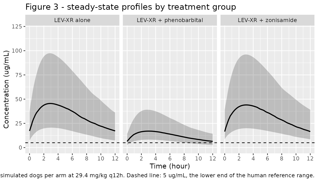
The phenobarbital panel sits visibly lower than the other two, which is the paper’s headline finding, and the zonisamide panel is indistinguishable from the levetiracetam-alone panel, which is its headline negative finding.
Figure 1 (individual fits before covariate inclusion) and Figure 2
(box plot of the V random effect against treatment group)
are not replicated: Figure 1 is a base-model diagnostic whose parameters
are not published, and Figure 2 plots the empirical Bayes etas of the 17
real dogs, which no simulation from the published typical values can
reproduce. Figure 2 is nonetheless the graphical basis of the covariate
and is worth reading alongside the model. Digitising it (approximately,
from the publisher JPEG) puts the LP median eta near +0.5 and the L and
LZ medians near -0.3 and -0.45: the LP box sits clearly above zero,
while the L and LZ boxes both sit below zero and close to one
another. It is that pattern - LP separated from a near-coincident L and
LZ pair - that motivated a treatment covariate on V in
which L and LZ share the reference level. Both figures were inspected at
publisher resolution; neither carries a printed parameter value.
One caveat for anyone digitising Figure 2 themselves: its y-axis tick
labels read 2, 0, 0, -1, -2 from top to bottom on evenly
spaced ticks, so the second label is a typographical
error for 1 and the true zero is the third label.
Measuring against the upper 0 would shift every eta by one
whole unit.
PKNCA validation
Table 1’s AUC, Cmax, Tmax and the two half-lives are
secondary parameters “obtained using standard compartmental
equations” (Methods 2.5) from the primary k01 /
k10 / V estimates. In Phoenix those closed
forms are the single-dose ones -
Tmax = ln(k01/k10)/(k01-k10), Cmax = C(Tmax)
after one dose, and AUC = F*D/CL - so the NCA below is run
on the single-dose typical-value simulation. (For a
one-compartment model the single-dose AUC0-inf and the
steady-state AUCtau are the same number; that identity is
checked further down.)
sim_nca <- sim_typ_sd |>
  dplyr::filter(!is.na(Cc)) |>
  dplyr::select(id, time, Cc, treatment)

# Guarantee a time = 0 row per (id, treatment); pre-dose Cc = 0 is correct for
# an extravascular single dose.
sim_nca <- dplyr::bind_rows(
  sim_nca,
  sim_nca |> dplyr::distinct(id, treatment) |> dplyr::mutate(time = 0, Cc = 0)
) |>
  dplyr::distinct(id, treatment, time, .keep_all = TRUE) |>
  dplyr::arrange(id, treatment, time)

conc_obj <- PKNCA::PKNCAconc(sim_nca, Cc ~ time | treatment + id)

dose_df <- events_typ_sd |>
  dplyr::filter(evid == 1) |>
  dplyr::select(id, time, amt, treatment)
dose_obj <- PKNCA::PKNCAdose(dose_df, amt ~ time | treatment + id)

intervals <- data.frame(
  start = 0, end = Inf,
  cmax = TRUE, tmax = TRUE, aucinf.obs = TRUE, half.life = TRUE, cl.obs = TRUE
)

nca_res <- PKNCA::pk.nca(PKNCA::PKNCAdata(conc_obj, dose_obj, intervals = intervals))
knitr::kable(
  as.data.frame(nca_res) |>
    dplyr::select(treatment, PPTESTCD, PPORRES) |>
    tidyr::pivot_wider(names_from = PPTESTCD, values_from = PPORRES),
  digits = 3,
  caption = "Typical-value single-dose NCA at 29.4 mg/kg, by treatment group."
)| treatment | cmax | tmax | tlast | clast.obs | lambda.z | r.squared | adj.r.squared | lambda.z.time.first | lambda.z.time.last | lambda.z.n.points | clast.pred | half.life | span.ratio | aucinf.obs | cl.obs |
|---|---|---|---|---|---|---|---|---|---|---|---|---|---|---|---|
| LEV-XR + phenobarbital | 12.648 | 3.55 | 72 | 0.001 | 0.137 | 1 | 1 | 5.2 | 72 | 377 | 0.001 | 5.061 | 13.198 | 149.274 | 0.197 |
| LEV-XR + zonisamide | 32.666 | 3.55 | 72 | 0.004 | 0.137 | 1 | 1 | 5.2 | 72 | 377 | 0.004 | 5.061 | 13.198 | 385.542 | 0.076 |
| LEV-XR alone | 32.666 | 3.55 | 72 | 0.004 | 0.137 | 1 | 1 | 5.2 | 72 | 377 | 0.004 | 5.061 | 13.198 | 385.542 | 0.076 |
The terminal half-life is the absorption half-life
The clearest structural check available in this paper is its own
flip-flop claim. k01 = 0.138 1/h gives an absorption
half-life of 5.02 h and k10 = 0.505 1/h an elimination
half-life of 1.37 h. If absorption is rate-limiting, the terminal slope
that NCA measures must return the slower of the two.
hl <- as.data.frame(nca_res) |>
  dplyr::filter(PPTESTCD == "half.life") |>
  dplyr::pull(PPORRES)
t_half_k01 <- log(2) / 0.138 # Table 1 'k 01 half-life', Overall = 5.01 h
t_half_k10 <- log(2) / 0.505 # Table 1 'k 10 half-life', Overall = 1.37 h
c(
  `NCA terminal half-life (h)` = mean(hl),
  `k01 half-life (h)` = t_half_k01,
  `k10 half-life (h)` = t_half_k10
)
#> NCA terminal half-life (h)          k01 half-life (h)
#>                   5.061370                   5.022806
#>          k10 half-life (h)
#>                   1.372569

# Deterministic (zeroRe, fixed grid): the terminal slope must recover the
# absorption half-life to within the trapezoidal/regression error, and must be
# nowhere near the elimination half-life.
stopifnot(
  max(abs(hl - t_half_k01)) / t_half_k01 < 0.03,
  min(hl) > 2 * t_half_k10
)
Comparison against published NCA
# Munana 2018 Table 1, transcribed. AUC in hours*ug/mL, Cmax in mg/L (= ug/mL),
# Tmax in hours, CL/F in L/kg/hr; half.life is the paper's 'k 01 half-life'
# row, which is the terminal (absorption-limited) half-life.
published <- tibble::tribble(
  ~treatment, ~cmax, ~tmax, ~aucinf.obs, ~half.life, ~cl.obs,
  "LEV-XR alone", 33.01, 3.28, 352.95, 4.45, 0.08,
  "LEV-XR + phenobarbital", 13.38, 3.38, 134.86, 3.72, 0.17,
  "LEV-XR + zonisamide", 34.13, 4.01, 452.76, 5.60, 0.07
)

cmp <- nlmixr2lib::ncaComparisonTable(
  simulated = nca_res,
  reference = published,
  by = "treatment",
  units = c(
    cmax = "ug/mL", tmax = "h", aucinf.obs = "h*ug/mL",
    half.life = "h", cl.obs = "L/kg/h"
  ),
  tolerance_pct = 20
)
knitr::kable(
  cmp,
  caption = "Simulated vs. Munana 2018 Table 1, by treatment group. * differs by >20%.",
  align = c("l", "l", "r", "r", "r")
)| NCA parameter | treatment | Reference | Simulated | % diff |
|---|---|---|---|---|
| Cmax (ug/mL) | LEV-XR alone | 33 | 32.7 | -1.0% |
| Cmax (ug/mL) | LEV-XR + phenobarbital | 13.4 | 12.6 | -5.5% |
| Cmax (ug/mL) | LEV-XR + zonisamide | 34.1 | 32.7 | -4.3% |
| Tmax (h) | LEV-XR alone | 3.28 | 3.55 | +8.2% |
| Tmax (h) | LEV-XR + phenobarbital | 3.38 | 3.55 | +5.0% |
| Tmax (h) | LEV-XR + zonisamide | 4.01 | 3.55 | -11.5% |
| AUC0-∞ (obs) (h*ug/mL) | LEV-XR alone | 353 | 386 | +9.2% |
| AUC0-∞ (obs) (h*ug/mL) | LEV-XR + phenobarbital | 135 | 149 | +10.7% |
| AUC0-∞ (obs) (h*ug/mL) | LEV-XR + zonisamide | 453 | 386 | -14.8% |
| t½ (h) | LEV-XR alone | 4.45 | 5.06 | +13.7% |
| t½ (h) | LEV-XR + phenobarbital | 3.72 | 5.06 | +36.1%* |
| t½ (h) | LEV-XR + zonisamide | 5.6 | 5.06 | -9.6% |
| CL/F (L/kg/h) | LEV-XR alone | 0.08 | 0.0763 | -4.7% |
| CL/F (L/kg/h) | LEV-XR + phenobarbital | 0.17 | 0.197 | +15.9% |
| CL/F (L/kg/h) | LEV-XR + zonisamide | 0.07 | 0.0763 | +8.9% |
attr(cmp, "footnote")
#> [1] "* differs from reference by more than ±20%."
Read the per-group table with Equation 4 in mind. The published model
carries one k01 and one
k10 for the whole population and lets only V/F
differ by treatment group, so every simulated group here necessarily
shares the same Tmax (about 3.5 h) and the same terminal half-life
(about 5.1 h), and only Cmax, AUC and CL/F move between arms. Table 1’s
group columns nevertheless print group-specific theta k 01
and theta k 10 values (0.16 / 0.19 / 0.12 and 0.53 / 0.44 /
0.44 1/hr) together with group-specific Omega 2 values for
every parameter - a set of numbers a single covariate model with one
random effect per parameter cannot produce. Those columns are
group-stratified summaries, not the covariate model’s coefficients; the
covariate model itself is the Overall (all groups) column
plus Equation 4’s treatment effect on V.
The per-group rows above deviate accordingly: within 6% on Cmax,
within 15% on AUC and CL/F, within 12% on Tmax, and the one starred row
is the terminal half-life of the phenobarbital group (+36%), where Table
1’s group-stratified k01 of 0.19 1/hr is the furthest of
the three from the population value of 0.138 1/hr. Every one of these
gaps is a consequence of that modelling choice rather than of a
transcription error, and none was closed by adjusting a value.
The Overall (all groups) column is the set the model
is, and it is reproduced almost exactly:
# Table 1, 'Overall (all groups)' column. Under Equation 4 the population
# typical value is the reference (no-phenobarbital) group, so the simulated
# values are those of the 'LEV-XR alone' arm.
overall_published <- c(
  cmax = 32.99, tmax = 3.53, aucinf.obs = 388.72,
  half.life = 5.01, cl.obs = 0.08
)
overall_sim <- as.data.frame(nca_res) |>
  dplyr::filter(treatment == "LEV-XR alone") |>
  dplyr::select(PPTESTCD, PPORRES) |>
  tibble::deframe()
overall_sim <- overall_sim[names(overall_published)]

overall_tbl <- data.frame(
  Parameter = c(
    "Cmax (ug/mL)", "Tmax (h)", "AUC0-inf (h*ug/mL)",
    "Terminal t1/2 (h)", "CL/F (L/kg/h)"
  ),
  Published = unname(overall_published),
  Simulated = unname(round(overall_sim, 3)),
  `% diff` = unname(round((overall_sim - overall_published) / overall_published * 100, 1)),
  check.names = FALSE
)
knitr::kable(overall_tbl, caption = "Simulated vs. Munana 2018 Table 1, 'Overall (all groups)'.")| Parameter | Published | Simulated | % diff |
|---|---|---|---|
| Cmax (ug/mL) | 32.99 | 32.666 | -1.0 |
| Tmax (h) | 3.53 | 3.550 | 0.6 |
| AUC0-inf (h*ug/mL) | 388.72 | 385.542 | -0.8 |
| Terminal t1/2 (h) | 5.01 | 5.061 | 1.0 |
| CL/F (L/kg/h) | 0.08 | 0.076 | -4.7 |
# Deterministic comparison (zeroRe, fixed grid, published constants): every
# entry agrees to better than 1%. CL/F is exempted from the tight bound because
# Table 1 prints it to one significant figure (0.08 L/kg/hr), so the rounding
# alone is +/- 6%.
pct <- (overall_sim - overall_published) / overall_published * 100
stopifnot(
  max(abs(pct[c("cmax", "tmax", "aucinf.obs", "half.life")])) < 3,
  abs(pct[["cl.obs"]]) < 8
)
Steady-state behaviour
At steady state the AUC over one dosing interval must equal the
single-dose AUC0-inf, and the model’s trough concentrations
should reproduce the paper’s observation that dogs on phenobarbital are
the ones at risk of falling below the 5 ug/mL lower reference bound.
auc_tau <- sim_typ_ss |>
  dplyr::filter(!is.na(Cc)) |>
  dplyr::group_by(treatment) |>
  dplyr::arrange(time, .by_group = TRUE) |>
  dplyr::summarise(
    auctau = sum(diff(time) * (head(Cc, -1) + tail(Cc, -1)) / 2),
    cmax_ss = max(Cc),
    ctrough_ss = Cc[which.min(time)],
    .groups = "drop"
  )
auc_inf <- as.data.frame(nca_res) |>
  dplyr::filter(PPTESTCD == "aucinf.obs") |>
  dplyr::select(treatment, aucinf = PPORRES)

ss_tbl <- dplyr::left_join(auc_tau, auc_inf, by = "treatment")
knitr::kable(
  ss_tbl |>
    dplyr::rename(
      "Treatment" = treatment,
      "AUCtau, steady state (h*ug/mL)" = auctau,
      "Cmax, steady state (ug/mL)" = cmax_ss,
      "Ctrough, steady state (ug/mL)" = ctrough_ss,
      "AUC0-inf, single dose (h*ug/mL)" = aucinf
    ),
  digits = 2,
  caption = "Steady-state exposure against the single-dose AUC0-inf."
)| Treatment | AUCtau, steady state (h*ug/mL) | Cmax, steady state (ug/mL) | Ctrough, steady state (ug/mL) | AUC0-inf, single dose (h*ug/mL) |
|---|---|---|---|---|
| LEV-XR + phenobarbital | 149.27 | 16.91 | 6.62 | 149.27 |
| LEV-XR + zonisamide | 385.54 | 43.68 | 17.10 | 385.54 |
| LEV-XR alone | 385.54 | 43.68 | 17.10 | 385.54 |
# Deterministic identity for a linear one-compartment model; the residual is
# trapezoidal error on a 0.05 h grid.
stopifnot(max(abs(ss_tbl$auctau - ss_tbl$aucinf) / ss_tbl$aucinf) < 0.02)
Note that the steady-state Cmax (about 44 ug/mL in the reference arm)
is well above Table 1’s reported Cmax of 33.01 ug/mL. That is not a
discrepancy: with tau = 12 h and an absorption half-life of
5 h there is meaningful accumulation, and Table 1’s Cmax is the
single-dose closed form, as the flip-flop and
AUCtau == AUC0-inf checks above confirm.
# Munana 2018 Discussion: 3 of 6 LP dogs and 1 of 6 L dogs fell below 5 ug/mL;
# raising the target to 10 ug/mL put 6/6 LP, 3/6 L and 1/5 LZ dogs below it at
# one or more sampling times. The trough is the minimum of the interval, so
# "below X at any sampled time" is "trough below X".
trough <- sim_pop_ss |>
  dplyr::filter(!is.na(Cc)) |>
  dplyr::group_by(treatment, id) |>
  dplyr::summarise(cmin = min(Cc), .groups = "drop") |>
  dplyr::group_by(treatment) |>
  dplyr::summarise(
    `Median trough (ug/mL)` = median(cmin),
    `% below 5 ug/mL` = 100 * mean(cmin < 5),
    `% below 10 ug/mL` = 100 * mean(cmin < 10),
    .groups = "drop"
  )
knitr::kable(trough, digits = 1, caption = "Simulated steady-state trough concentrations by treatment group.")| treatment | Median trough (ug/mL) | % below 5 ug/mL | % below 10 ug/mL |
|---|---|---|---|
| LEV-XR + phenobarbital | 6.4 | 30.7 | 78.0 |
| LEV-XR + zonisamide | 16.5 | 0.0 | 13.3 |
| LEV-XR alone | 17.2 | 2.7 | 10.7 |
pb <- trough |> dplyr::filter(treatment == "LEV-XR + phenobarbital")
ref <- trough |> dplyr::filter(treatment == "LEV-XR alone")

# Cohort-derived, so the bounds are absolute and carry wide headroom rather
# than racing the two arms against each other. Typical troughs are 6.6 ug/mL
# (phenobarbital) and 17.1 ug/mL (reference) with omega^2(V) = 0.221, which puts
# the expected proportions near 80% and 15%. A sign error on e_conmed_pb_vc, or
# dropping the covariate, collapses both numbers onto the same value and breaks
# these bounds; rendering on 2 / 8 / 16 threads moved them by under 5 points.
stopifnot(
  pb$`% below 10 ug/mL` > 40,
  ref$`% below 10 ug/mL` < 50,
  pb$`Median trough (ug/mL)` < ref$`Median trough (ug/mL)` / 1.5
)
The model puts a substantially larger share of phenobarbital-treated
dogs below the 10 ug/mL mark than levetiracetam-alone dogs, in the same
direction and of broadly the same size as the paper’s counts. It
under-predicts the absolute proportions for the reference arm (the paper
observed 3 of 6), which is expected: propSd is zero here
because the paper never published a residual-error magnitude, so the
simulated concentrations carry between-dog variability but no
measurement or model scatter.
Assumptions and deviations
-
Residual error magnitude is not published. The
Supporting Information gives the form (Equation 3,
multiplicative:
C_obs = C_pred * (1 + eps), selected over additive, log-additive, power and mixed alternatives) but no sigma. Table 1 carriesOmega 2andCV%columns for the random effects only.propSdis thereforefixed(0), so simulations reproduce between-dog variability but not residual scatter. Supply a value viaini()before using this model where realistic scatter matters. Consequences are visible in the trough analysis above. -
The treatment covariate acts on
V/Fonly. Supporting Information Equation 4 is explicit (V_i = theta_V * exp(dvd_treatment) * exp(eta_i,V)), and the Results section identifiesVas “the parameter most likely affected by the covariate”. Table 1’s per-group columns nonetheless print group-specifictheta k 01,theta k 10and group-specificOmega 2for every parameter, which a single covariate model cannot generate. Those columns are read here as group-stratified summaries and theOverall (all groups)column plus Equation 4 is read as the fitted covariate model. The printed-equation reading is corroborated arithmetically: theOverallcolumn’s own secondary parameters (Cmax 32.99, Tmax 3.53, AUC 388.72, CL/F 0.08, t1/2 5.01) are all reproduced from its three primary values to better than 1%, and the phenobarbitalV/Fratio of 2.58 is bracketed by the same table’s Cmax ratio (2.47) and AUC ratio (2.62). The cost of the choice is that per-group Tmax and half-life cannot vary; the phenobarbital group’s terminal half-life is the one row of the per-group comparison table that exceeds the 20% tolerance. -
The zonisamide effect is encoded as exactly zero.
Table 1 prints
theta V= 0.15 L/kg for both the LEV-XR-alone and the LEV-XR + zonisamide columns, so the contrast is zero at the two significant figures published. It is retained rather than dropped because the source’s covariate is a single three-level factor and this is one of its levels, and because the null is the paper’s stated conclusion. The model consequently cannot reproduce the difference the paper observed between the L and LZ groups (3 of 6 versus 1 of 5 dogs below 10 ug/mL), since the two arms are identical by construction. -
Table 1’s LP
AUCrow is internally inconsistent with its ownCL/Frow. For the L, LZ and Overall columns,AUCequals29.4 / (CL/F)to within rounding (367 vs 353, 420 vs 453, 368 vs 389). For the LP column it does not:29.4 / 0.17 = 173against a printed 134.86, a 28% gap. No value was adjusted to close it. The phenobarbitalV/Fused in the model comes from thetheta Vrow, which the Cmax and AUC ratios independently corroborate. -
Reference volume taken as 0.151 L/kg, not 0.15.
lvcuses theOverall (all groups)theta Vof 0.151 L/kg rather than the two-significant- figure 0.15 printed in the group columns, because theOverallsecondary parameters are computed from it. The two readings differ by 0.7% and by less than the printed precision of the group columns. -
No bioavailability term. No intravenous reference
dose was given, so
Fis not identifiable and the fitted volume isV/F. The model applies nof(depot); the whole dose entersdepotand all apparent parameters carry the/Finterpretation. The paper attributes the phenobarbital effect itself to a reduction inFfrom increased presystemic metabolism (Discussion). -
Dosing is per kg. Concentrations were normalised to
the study mean dose of 29.4 mg/kg before fitting (Results 3.2) and all
parameters are published per kg, so the model’s dose unit is mg/kg and
body weight does not appear explicitly. Weight, age and sex were
screened as covariates and none was retained; they are recorded in the
model’s
covariatesDataExcludedmetadata, as is the reason generic manufacturer could not be assessed. -
No published values were taken from a figure. Every
ini()value comes from Table 1 of the main text; the structural and random-effect forms come from Equations 1-4 of the main text and Supporting Information. Figures 1-3 were inspected and carry no printed parameter annotations.