Upadacitinib in axial spondyloarthritis (Bhatnagar 2024)
Source:vignettes/articles/Bhatnagar_2024_upadacitinib.Rmd
Bhatnagar_2024_upadacitinib.RmdModels and source
Bhatnagar 2024 reports a population pharmacokinetic model and four exposure-response models built on the SELECT-AXIS 1 and SELECT-AXIS 2 trials of upadacitinib in axial spondyloarthritis (axSpA). Following the package’s policy of replicating the authors’ model structure, each is a separate model file and all five share this vignette.
| Model | Endpoint | Structure | Source |
|---|---|---|---|
Bhatnagar_2024_upadacitinib |
plasma concentration | 2-compartment, parallel zero-order + first-order absorption with lag, linear elimination | Table S3 and the Appendix S1 control streams |
Bhatnagar_2024_upadacitinib_asas20_as |
P(ASAS20 at week 14), AS | logistic, treatment indicator only | Table S4 |
Bhatnagar_2024_upadacitinib_asas40_as |
P(ASAS40 at week 14), AS | logistic, treatment indicator only | Table S4 |
Bhatnagar_2024_upadacitinib_asas20_nraxspa |
P(ASAS20 at week 14), nr-axSpA | logistic, treatment indicator only | Table S4 |
Bhatnagar_2024_upadacitinib_asas40_nraxspa |
P(ASAS40 at week 14), nr-axSpA | logistic, treatment indicator only | Table S4 |
- Citation: Bhatnagar S, Eckert D, Stodtmann S, Song I-H, Wung P, Liu W, Mohamed M-EF. Population pharmacokinetics and exposure-response analyses for efficacy and safety of upadacitinib in patients with axial spondyloarthritis. Clin Transl Sci. 2024;17(2):e13733. doi:10.1111/cts.13733. Parameter values are Table S3 and the SELECT-AXIS-2 NONMEM control stream in Appendix S1 of the Supporting Information. The fixed structural parameters and covariate coefficients originate in the upstream pooled healthy-volunteer / rheumatoid-arthritis population PK model of Klunder B, Mittapalli RK, Mohamed M-EF, et al. (Bhatnagar 2024 reference 17), which is not itself in nlmixr2lib; the related earlier phase I/II analysis is available as modellib(‘Klunder_2017_upadacitinib’).
- Article: https://doi.org/10.1111/cts.13733
- Supporting Information (Tables S1-S4, Figures S1-S2, and the NONMEM control streams in Appendix S1) is open access alongside the article.
# readModelDb() returns the raw model FUNCTION, not a parsed model, so it is
# wrapped in rxode2::rxode() once here. Everything downstream (zeroRe(), ini(),
# rxSolve(), $population) needs the parsed rxUi object.
mod_pk   <- rxode2::rxode(readModelDb("Bhatnagar_2024_upadacitinib"))
mod_2_as <- rxode2::rxode(readModelDb("Bhatnagar_2024_upadacitinib_asas20_as"))
mod_4_as <- rxode2::rxode(readModelDb("Bhatnagar_2024_upadacitinib_asas40_as"))
mod_2_nr <- rxode2::rxode(readModelDb("Bhatnagar_2024_upadacitinib_asas20_nraxspa"))
mod_4_nr <- rxode2::rxode(readModelDb("Bhatnagar_2024_upadacitinib_asas40_nraxspa"))
What was actually estimated here
This is a sequential, inherited model, and reading it any other way will mislead. The structural parameters and every covariate coefficient were fixed from a previously published upadacitinib population PK model built on 4170 healthy volunteers and patients with rheumatoid arthritis (Bhatnagar 2024 reference 17). Only three things were re-estimated, and only once, on the SELECT-AXIS 1 ankylosing spondylitis data:
- the apparent central volume
Vc/F(171 L, against 156 L in the source model), which the authors re-estimated because it “improved the stability of the model in terms of successful estimation and covariance steps”; - the interindividual variability;
- the residual error.
The SELECT-AXIS 2 run then held everything fixed – its
control stream is a MAXEVAL=0 evaluation. So the file in
this package is a faithful copy of a model that was, in this paper,
almost entirely asserted rather than fitted. fixed() in
ini() marks exactly the rows Table S3 flags
(FIX).
The four exposure-response models carry an equally important caveat, discussed under Exposure-response below: none of them contains an exposure term.
Population
The population pharmacokinetic datasets comprised 173 patients with ankylosing spondylitis (AS) and 71 patients with non-radiographic axial spondyloarthritis (nr-axSpA), pooled from SELECT-AXIS 1 (NCT03178487) and the two standalone studies of SELECT-AXIS 2 (NCT04169373). PK samples were drawn in every SELECT-AXIS 1 patient and in about 30% of SELECT-AXIS 2 patients, at weeks 2, 8, 12 and 14; the assay lower limit of quantitation was 0.05 ng/mL and below-limit samples were imputed at LLOQ/2 (the M5 method).
Among the 295 randomized subjects with PK sampling scheduled (Table S1), median age was 44 years (range 19-82), median body weight 79.0 kg (range 41.5-144), and 45% were female. The exposure-response analyses used a larger cohort – 339 patients with AS and 143 with nr-axSpA, 482 in total (Table S2) – because efficacy and safety were collected in everyone. The two sub-populations differ sharply in sex balance: the AS cohort is 28% female while the nr-axSpA cohort is 64% female.
In all three studies patients were randomized 1:1 to upadacitinib 15 mg once daily (extended-release tablet) or placebo, with the primary ASAS40 end point at week 14.
The same information is available programmatically:
str(readModelDb("Bhatnagar_2024_upadacitinib")()$population, max.level = 1)
#> List of 14
#>  $ species       : chr "human"
#>  $ n_subjects    : int 244
#>  $ n_studies     : int 3
#>  $ age_range     : chr "19-82 years (subjects with PK sampling, Table S1)"
#>  $ age_median    : chr "44 years (subjects with PK sampling, Table S1; mean 45, SD 13)"
#>  $ weight_range  : chr "41.5-144 kg (subjects with PK sampling, Table S1)"
#>  $ weight_median : chr "79.0 kg (subjects with PK sampling, Table S1; mean 81.2, SD 20.0). The covariate reference weight of 74 kg is i"| __truncated__
#>  $ sex_female_pct: num 45
#>  $ race_ethnicity: chr "Not tabulated. Bhatnagar 2024 Figure 4 compares model-estimated average concentrations between Asian and non-As"| __truncated__
#>  $ disease_state : chr "Axial spondyloarthritis. The population PK datasets comprised 173 patients with ankylosing spondylitis (SELECT-"| __truncated__
#>  $ dose_range    : chr "Upadacitinib 15 mg once daily, extended-release tablet, versus placebo (1:1 randomization) through the week-14 "| __truncated__
#>  $ regions       : chr "Multinational phase II/III programme; not broken out in Bhatnagar 2024."
#>  $ renal_function: chr "Creatinine clearance was a retained covariate on apparent oral clearance; Bhatnagar 2024 reports that plasma ex"| __truncated__
#>  $ notes         : chr "Clinical trial registrations NCT03178487 (SELECT-AXIS 1) and NCT04169373 (SELECT-AXIS 2 studies 1 and 2). PK sa"| __truncated__
Source trace
The per-parameter origin is recorded as an in-file comment next to
each ini() entry. The table below collects them in one
place.
Population pharmacokinetics
(Bhatnagar_2024_upadacitinib)
| Parameter | Value | Fixed? | Source location |
|---|---|---|---|
lcl (CL/F) |
40.9 L/h | fixed | Table S3; control-stream THETA(1) = 3.71 |
lvc (Vc/F) |
171 L | estimated | Table S3, 95% CI 128-227; THETA(2) = 5.14 |
lq (Q/F) |
3.22 L/h | fixed | Table S3; THETA(10) = 1.17 |
lvp (Vp/F) |
68.0 L | fixed | Table S3; THETA(11) = 4.22 |
lka_er |
0.0523 1/h | fixed | Table S3 “Extended-Release KA”; THETA(3) = -2.95 |
ltlag_er |
0.154 h | fixed | Table S3 “Extended-Release Lag time”; THETA(4) =
-1.87 |
logitalpha |
74.5% | fixed | Table S3 “Fraction … Zero-Order Process”; THETA(5) =
1.07, entering as EXP(t)/(1+EXP(t))
|
ld2 |
3.29 h | fixed | Table S3 “Zero-Order Infusion Duration”; THETA(6) =
1.19 |
lka_ir |
2.77 1/h | fixed | Table S3 “Immediate-Release KA”; THETA(7) = 1.02 |
ltlag_ir |
0.200 h | fixed | control-stream THETA(8) = -1.61 (Table S3 misprints
2.00; see Errata) |
lfrel_er |
76.2% | fixed | Table S3 “Bioavailability … Relative to the Immediate-Release”;
THETA(9) = -0.272 |
e_crcl_cl |
0.256 | fixed | Table S3; THETA(13)
|
e_wt_cl |
0.132 | fixed | Table S3; THETA(15)
|
e_wt_vc |
0.804 | fixed | Table S3; THETA(14)
|
e_patient_cl |
0.754 | fixed | Table S3 “CL/F Ratio of Diseased Patients …”;
THETA(12)
|
etalcl, etalvc block |
0.111 / -0.160 / 0.593 | estimated | control-stream $OMEGA BLOCK(2); Table S3 reports only
the diagonal as 33% and 77% |
etalka_er |
0.643 | estimated | control-stream second $OMEGA; Table S3 “IIV on
Extended-Release KA” 80% |
propSd |
0.559 | estimated | Table S3; $SIGMA 3.12e-01 |
addSd |
0.00244 ng/mL | estimated | Table S3; $SIGMA 5.95e-06 |
| Reference CrCL / weight | 108.70 mL/min / 74 kg | – | control-stream LOG(CRCL/108.70),
LOG(WTKG/74)
|
ODE structure,
F1/F2/D2/ALAG
|
n/a | – | Appendix S1 $PK block (NONMEM ADVAN4) |
| Residual-error form | combined | – | Appendix S1 $ERROR:
Y = IPRED + IPRED*EPS(1) + EPS(2)
|
Exposure-response (four logistic models)
| Model | Intercept | Treatment coefficient | Source location |
|---|---|---|---|
..._asas20_as |
-0.456 (95% CI -0.769, -0.143) | 0.924 (0.487, 1.36), p = 3.44e-5 | Table S4 |
..._asas40_as |
-1.31 (-1.69, -0.939) | 1.06 (0.579, 1.54), p = 1.47e-5 | Table S4 |
..._asas20_nraxspa |
-0.511 (-0.988, -0.0337) | 1.18 (0.498, 1.87), p = 7.15e-4 | Table S4 |
..._asas40_nraxspa |
-1.17 (-1.72, -0.630) | 0.745 (0.0224, 1.47), p = 0.0433 | Table S4 |
| model form (all four) | n/a | n/a | Bhatnagar 2024 Equation 3 |
Virtual cohort
Original observed data are not publicly available. The cohort below approximates the published trial demographics (Table S2) for each indication, 200 subjects per arm.
Creatinine clearance is the one required covariate the paper never tabulates. It is derived here with the Cockcroft-Gault formula from the simulated age, weight and sex plus a plausible serum-creatinine distribution – see Assumptions and deviations.
# set.seed() seeds R's RNG for the covariate draws. It does NOT seed rxode2's
# simulation RNG, whose streams are partitioned per solver thread, so the
# between-subject draws differ between this machine and CI. Every assertion
# below is therefore written on medians and on structural identities, never on
# the extremes of a random cohort.
set.seed(20240213)
rxode2::rxSetSeed(20240213)

N_ARM <- 200L

make_cohort <- function(n, wt_mean, wt_sd, wt_lo, wt_hi, pct_female,
                        indication, id_offset = 0L) {
  wt   <- pmin(pmax(rnorm(n, wt_mean, wt_sd), wt_lo), wt_hi)
  age  <- pmin(pmax(rnorm(n, 45, 13), 19), 82)
  sexf <- rbinom(n, 1L, pct_female / 100)
  # Serum creatinine is not reported either; a log-normal centred on
  # 0.85 mg/dL with 18% CV is a conventional adult distribution.
  scr  <- exp(rnorm(n, log(0.85), 0.18))
  crcl <- ((140 - age) * wt / (72 * scr)) * ifelse(sexf == 1L, 0.85, 1)

  tibble(
    id          = id_offset + seq_len(n),
    WT          = wt,
    CRCL        = pmin(pmax(crcl, 30), 250),
    DIS_HEALTHY = 0,      # every SELECT-AXIS subject is a patient
    FORM_UPA_ER = 1,      # every SELECT-AXIS subject received the ER tablet
    indication  = indication
  )
}

subjects <- bind_rows(
  # Table S2, AS column: weight mean 80.4 (SD 19.0), range 41.5-156; 28% female
  make_cohort(N_ARM, 80.4, 19.0, 41.5, 156, 28, "AS", id_offset = 0L),
  # Table S2, nr-axSpA column: mean 81.1 (SD 19.5), range 49.3-144; 64% female
  make_cohort(N_ARM, 81.1, 19.5, 49.3, 144, 64, "nr-axSpA", id_offset = N_ARM)
)

summary(subjects$WT)
#>    Min. 1st Qu.  Median    Mean 3rd Qu.    Max.
#>   41.50   67.15   80.70   80.49   92.80  139.89
summary(subjects$CRCL)
#>    Min. 1st Qu.  Median    Mean 3rd Qu.    Max.
#>    30.0    88.9   114.7   116.3   139.4   250.0
Building the event table
The extended-release absorption is a parallel
process, so each administration is two dose records at
the same time: one into depot (the first-order arm, scaled
by f(depot)) and one into central with
rate = -2 (rxode2’s modelled-duration flag, giving the
zero-order arm over dur(central)). Observation records
point at cmt = "central" – the ODE state, never the
algebraic observable Cc.
DOSE_TIMES <- seq(0, 672, by = 24)      # 29 once-daily doses, days 1-29
OBS_TIMES  <- seq(672, 696, by = 0.25)  # the 29th dosing interval

expand_rows <- function(df, times) df[rep(seq_len(nrow(df)), each = length(times)), ]

depot_doses <- expand_rows(subjects, DOSE_TIMES) |>
  mutate(time = rep(DOSE_TIMES, nrow(subjects)),
         amt = 15, evid = 1L, cmt = "depot", rate = 0)

# Same nominal amount into central; f(central) applies the zero-order share and
# dur(central) the 3.29 h duration.
central_doses <- depot_doses |> mutate(cmt = "central", rate = -2)

observations <- expand_rows(subjects, OBS_TIMES) |>
  mutate(time = rep(OBS_TIMES, nrow(subjects)),
         amt = NA_real_, evid = 0L, cmt = "central", rate = 0)

events <- bind_rows(depot_doses, central_doses, observations) |>
  arrange(id, time, desc(evid))

# Multi-cohort guard: IDs must be disjoint across the two arms.
stopifnot(!anyDuplicated(unique(events[, c("id", "time", "evid", "cmt")])))
stopifnot(length(unique(events$id)) == 2 * N_ARM)Replicate published figures
# Replicates the shape of Figure 1 of Bhatnagar 2024: observed upadacitinib
# concentrations versus time since last dose, by indication, with the median
# and the 5th/95th percentiles.
sim |>
  mutate(tsld = time - max(DOSE_TIMES)) |>
  group_by(indication, tsld) |>
  summarise(Q05 = quantile(Cc, 0.05), Q50 = median(Cc), Q95 = quantile(Cc, 0.95),
            .groups = "drop") |>
  ggplot(aes(tsld, Q50)) +
  geom_ribbon(aes(ymin = Q05, ymax = Q95), alpha = 0.2) +
  geom_line(linewidth = 0.8) +
  facet_wrap(~indication) +
  scale_x_continuous(breaks = seq(0, 24, by = 4)) +
  labs(x = "Time since last dose (h)", y = "Upadacitinib concentration (ng/mL)",
       title = "Steady-state profile, upadacitinib 15 mg once daily",
       caption = paste("Median and 5th-95th percentile band of a simulated cohort.",
                       "Compare with Figure 1 of Bhatnagar 2024."))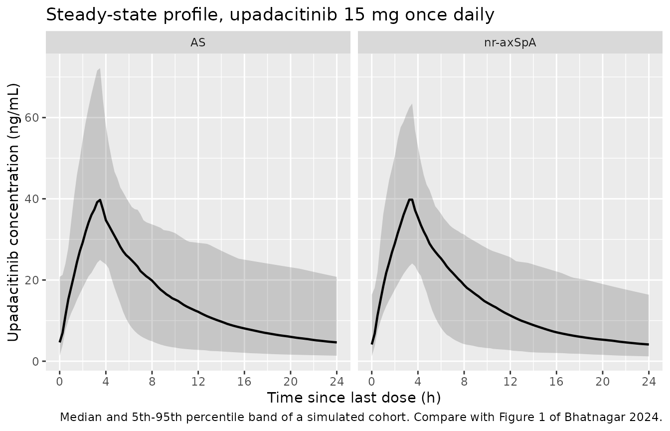
The peak sits just after 3 h, which is where the model puts it by construction: the zero-order arm carries 74.5% of the absorbed dose and runs from the 0.154 h lag to 0.154 + 3.29 = 3.44 h. That is inside the “2 to 4 h” window the paper quotes for the extended-release tablet.
PKNCA validation
Steady-state NCA over the 29th dosing interval. Terminal half-life is
deliberately not requested: absorption is the slow step
here – the extended-release Ka of 0.0523 1/h is a 13.3 h
absorption half-life against a much faster disposition, so the profile
is flip-flop – and a 24 h window on such a profile
under full interindividual variability yields a heavily
NA-poisoned, tmax-selected estimate. Table 1 reports no
half-life to compare against in any case.
sim_nca <- sim |>
  dplyr::filter(!is.na(Cc)) |>
  dplyr::select(id, time, Cc, indication)

conc_obj <- PKNCA::PKNCAconc(sim_nca, Cc ~ time | indication + id)

dose_df <- events |>
  dplyr::filter(evid == 1, cmt == "depot") |>
  dplyr::select(id, time, amt, indication)

dose_obj <- PKNCA::PKNCAdose(dose_df, amt ~ time | indication + id)

intervals <- data.frame(
  start   = 672,
  end     = 696,
  cmax    = TRUE,
  tmax    = TRUE,
  auclast = TRUE,
  cav     = TRUE
)

nca_res <- PKNCA::pk.nca(PKNCA::PKNCAdata(conc_obj, dose_obj, intervals = intervals))Ctrough is read directly, not taken from
cmin
PKNCA’s own ctrough returns NA for every
subject under this interval / dosing layout, so the end-of-interval
concentration is read straight off the solved profile. That is a value
lookup, not an alternative NCA rule, and it is deliberately
not cmin: absorption here is delayed by a
0.154 h lag and then dominated by a 3.29 h zero-order input, so the
minimum concentration over a dosing interval sits at the interval
start (immediately after the dose, before any drug has been
absorbed) rather than at its end. The two happen to agree to about 0.2%
at steady state, but cmin is the wrong instrument for an
extravascular trough on principle and is not used.
ctrough_df <- sim |>
  dplyr::filter(time == max(OBS_TIMES)) |>
  dplyr::transmute(indication, id, PPTESTCD = "ctrough", PPORRES = Cc)

nca_long <- dplyr::bind_rows(
  as.data.frame(nca_res)[, c("indication", "id", "PPTESTCD", "PPORRES")],
  ctrough_df
)

stopifnot(!anyNA(nca_long$PPORRES))

nca_med <- nca_long |>
  group_by(indication, PPTESTCD) |>
  summarise(median = median(PPORRES),
            p05    = quantile(PPORRES, 0.05),
            p95    = quantile(PPORRES, 0.95),
            .groups = "drop")

nca_med |>
  mutate(across(c(median, p05, p95), ~ signif(., 3))) |>
  dplyr::rename("Indication" = indication, "Parameter" = PPTESTCD,
                "Median" = median, "5th pctile" = p05, "95th pctile" = p95) |>
knitr::kable(caption = "Simulated steady-state NCA by indication.")| Indication | Parameter | Median | 5th pctile | 95th pctile |
|---|---|---|---|---|
| AS | auclast | 345.00 | 206.000 | 613.0 |
| AS | cav | 14.40 | 8.590 | 25.5 |
| AS | cmax | 41.60 | 22.500 | 67.9 |
| AS | ctrough | 3.96 | 0.983 | 17.9 |
| AS | tmax | 3.50 | 3.250 | 3.5 |
| nr-axSpA | auclast | 365.00 | 212.000 | 662.0 |
| nr-axSpA | cav | 15.20 | 8.850 | 27.6 |
| nr-axSpA | cmax | 41.40 | 25.100 | 63.9 |
| nr-axSpA | ctrough | 4.85 | 0.998 | 17.6 |
| nr-axSpA | tmax | 3.50 | 3.250 | 3.5 |
Comparison against Table 1 of Bhatnagar 2024
Table 1 reports model-estimated steady-state exposures for the 15 mg once-daily regimen as median (5th to 95th percentile).
published <- tibble::tribble(
  ~indication, ~cmax, ~cav,  ~auclast, ~ctrough,
  "AS",         38.8,  14.5,  348,      3.71,
  "nr-axSpA",   37.3,  14.8,  355,      4.58
)

cmp <- nlmixr2lib::ncaComparisonTable(
  simulated = nca_long,
  reference = published,
  by        = "indication",
  units     = c(cmax = "ng/mL", cav = "ng/mL",
                auclast = "ng*h/mL", ctrough = "ng/mL"),
  tolerance_pct = 20
)

knitr::kable(
  cmp,
  caption = "Simulated vs. Bhatnagar 2024 Table 1. * differs from reference by >20%.",
  align   = c("l", "l", "r", "r", "r")
)| NCA parameter | indication | Reference | Simulated | % diff |
|---|---|---|---|---|
| Cmax (ng/mL) | AS | 38.8 | 41.6 | +7.1% |
| Cmax (ng/mL) | nr-axSpA | 37.3 | 41.4 | +11.0% |
| AUClast (ng*h/mL) | AS | 348 | 345 | -0.9% |
| AUClast (ng*h/mL) | nr-axSpA | 355 | 365 | +2.9% |
| Cavg (ng/mL) | AS | 14.5 | 14.4 | -0.9% |
| Cavg (ng/mL) | nr-axSpA | 14.8 | 15.2 | +2.8% |
| Ctrough (ng/mL) | AS | 3.71 | 3.96 | +6.6% |
| Ctrough (ng/mL) | nr-axSpA | 4.58 | 4.85 | +5.8% |
# Structural gate on the CENTRE of the distribution. A mis-transcribed
# clearance, dose, bioavailability or unit moves every median by tens of
# percent; the extremes of a random cohort are not reproducible across rxode2
# builds and are not gated. Observed spread of |pct| when this vignette was
# written: cav 1.8-5.0%, auclast 1.8-5.1%, cmax 5.2-6.2%, ctrough 4.2-11.4%.
gate <- nca_med |>
  dplyr::select(indication, PPTESTCD, median) |>
  tidyr::pivot_wider(names_from = PPTESTCD, values_from = median) |>
  dplyr::left_join(published, by = "indication", suffix = c("_sim", "_pub")) |>
  dplyr::mutate(
    pct_cav     = 100 * (cav_sim / cav_pub - 1),
    pct_auc     = 100 * (auclast_sim / auclast_pub - 1),
    pct_cmax    = 100 * (cmax_sim / cmax_pub - 1),
    pct_ctrough = 100 * (ctrough_sim / ctrough_pub - 1)
  )

stopifnot(
  # C_avg depends ONLY on clearance and relative bioavailability, both fixed,
  # so this is the tightest available check on the structural transcription.
  all(abs(gate$pct_cav) < 20),
  all(abs(gate$pct_auc) < 20),
  # C_max additionally involves Vc and Ka, so it is looser.
  all(abs(gate$pct_cmax) < 25),
  # C_trough is the most variable published quantity.
  all(abs(gate$pct_ctrough) < 30)
)

# Peak timing: the paper quotes 2-4 h for the extended-release tablet.
tmax_med <- nca_med |> dplyr::filter(PPTESTCD == "tmax") |> dplyr::pull(median)
stopifnot(all(tmax_med >= 2), all(tmax_med <= 5))

gate |>
  dplyr::select(indication, pct_cav, pct_auc, pct_cmax, pct_ctrough) |>
  dplyr::mutate(dplyr::across(dplyr::where(is.numeric), ~ round(., 1))) |>
knitr::kable(caption = "Percent difference of the simulated median from Table 1.")| indication | pct_cav | pct_auc | pct_cmax | pct_ctrough |
|---|---|---|---|---|
| AS | -0.9 | -0.9 | 7.1 | 6.6 |
| nr-axSpA | 2.8 | 2.9 | 11.0 | 5.8 |
The simulated 5th-95th interval for Cmax is
wider than the published one (roughly 26-68 against
27.7-51.4 ng/mL) while Cavg and AUC match closely at both
tails. That asymmetry is expected and is not a transcription problem.
Bhatnagar 2024 derived its Table 1 percentiles from post hoc
empirical Bayesian estimates under a sparse sampling scheme (four
samples, largely troughs). Cavg is a function of clearance
alone, whose 33% interindividual variability is well informed by trough
data, so its EBE distribution is close to the true one. Cmax
additionally depends on Vc/F (77% IIV) and the
extended-release Ka (80% IIV), neither of which sparse
trough sampling can identify, so those EBEs shrink hard toward the
typical value and the published spread is correspondingly compressed. A
forward simulation draws from the full omega and cannot reproduce
shrinkage.
Internal structural identities
At steady state, C_avg = F_rel * Dose / (CL * tau).
Recovering that from the integrated profile confirms that the
bioavailability split, the zero-order duration and the covariate model
all conserve mass, and it is independent of anything the paper published
– it tests the encoding against itself.
The check is run twice, with deliberately different bounds.
Typical values first. With the random effects zeroed there is no draw at all, so the only error is numerical and the bound can be tight.
typical <- tibble(
  id = 1:9,
  WT = rep(c(50, 74, 120), times = 3),
  CRCL = rep(c(60, 108.7, 180), each = 3),
  DIS_HEALTHY = 0, FORM_UPA_ER = 1
)

typ_events <- bind_rows(
  expand_rows(typical, DOSE_TIMES) |>
    mutate(time = rep(DOSE_TIMES, nrow(typical)), amt = 15, evid = 1L,
           cmt = "depot", rate = 0),
  expand_rows(typical, DOSE_TIMES) |>
    mutate(time = rep(DOSE_TIMES, nrow(typical)), amt = 15, evid = 1L,
           cmt = "central", rate = -2),
  expand_rows(typical, OBS_TIMES) |>
    mutate(time = rep(OBS_TIMES, nrow(typical)), amt = NA_real_, evid = 0L,
           cmt = "central", rate = 0)
) |> arrange(id, time, desc(evid))

# zeroRe() strips omega on purpose, so rxode2 notes a multi-subject solve with
# no between-subject variability. That is the intent.
typ_chk <- suppressWarnings(
  as.data.frame(rxode2::rxSolve(rxode2::zeroRe(mod_pk), typ_events))
) |>
  group_by(id) |>
  summarise(cav = sum(diff(time) * (head(Cc, -1) + tail(Cc, -1)) / 2) / 24,
            cl = first(cl), .groups = "drop") |>
  mutate(pct = 100 * (cav / (0.762 * 15 * 1000 / (cl * 24)) - 1))
#> ℹ omega/sigma items treated as zero: 'etalcl', 'etalvc', 'etalka_er'

# Observed maximum 0.013% across this 3x3 weight-by-renal-function grid.
stopifnot(max(abs(typ_chk$pct)) < 0.1)
signif(range(typ_chk$pct), 3)
#> [1] 0.00533 0.01260
Then the full cohort, on the median and a robust
quantile – deliberately not on the maximum.
Interindividual variability is 80% on the extended-release
Ka and 77% on Vc/F, so a 400-subject draw
reliably contains a few subjects whose absorption half-life runs to
several days and which are therefore still approaching steady state even
at day 29. Those subjects put a heavy tail on the deviation: across
independent draws of this same cohort the maximum ranged from 0.7% to
8.2% while the median stayed at 0.008% and the 95th percentile at 0.05%.
A max() bound here would be an assertion on the extreme of
a random cohort, which is exactly the shape that passes locally and
fails in CI.
cl_per_id <- sim |> group_by(id) |> summarise(cl = first(cl), .groups = "drop")

cav_sim <- nca_long |>
  dplyr::filter(PPTESTCD == "cav") |>
  dplyr::select(id, cav = PPORRES) |>
  dplyr::mutate(id = as.integer(as.character(id))) |>
  dplyr::left_join(cl_per_id, by = "id") |>
  dplyr::mutate(closed_form = 0.762 * 15 * 1000 / (cl * 24),
                pct = 100 * (cav / closed_form - 1))

# Observed across three independent draws: median +0.008%, p95 0.046-0.054%.
# The bounds below sit an order of magnitude clear of that and still go red if
# the mass balance or the bioavailability split is wrong.
stopifnot(
  abs(median(cav_sim$pct)) < 0.5,
  quantile(abs(cav_sim$pct), 0.95) < 1
)
signif(quantile(abs(cav_sim$pct), c(0.5, 0.9, 0.95, 0.99)), 3)
#>     50%     90%     95%     99%
#> 0.00218 0.03280 0.06150 0.16200
# The formulation switch changes only absorption, never clearance, so for the
# same dose AUC_inf(ER) / AUC_inf(IR) must equal the relative bioavailability
# 0.762 exactly. This is the sharpest available test of FORM_UPA_ER.
single_dose <- function(form, id_offset) {
  s <- tibble(id = id_offset + 1:3, WT = c(60, 74, 100), CRCL = c(80, 108.7, 140),
              DIS_HEALTHY = 0, FORM_UPA_ER = form)
  ot <- seq(0, 240, by = 0.05)
  dep <- s |> mutate(time = 0, amt = 15, evid = 1L, cmt = "depot", rate = 0)
  obs <- s[rep(1:3, each = length(ot)), ] |>
    mutate(time = rep(ot, 3), amt = NA_real_, evid = 0L, cmt = "central", rate = 0)
  # With FORM_UPA_ER = 0 the zero-order share alpha is 0, so the central dose
  # record is unnecessary (and would be a zero-amount modelled-duration dose).
  ev <- if (form == 1) {
    bind_rows(dep, dep |> mutate(cmt = "central", rate = -2), obs)
  } else {
    bind_rows(dep, obs)
  }
  arrange(ev, id, time, desc(evid))
}

trapz_auc <- function(d) {
  d |> group_by(id) |>
    summarise(auc = sum(diff(time) * (head(Cc, -1) + tail(Cc, -1)) / 2), .groups = "drop")
}

mod_typ <- rxode2::zeroRe(mod_pk)
# zeroRe() strips omega on purpose (these are typical-value evaluations), so
# rxode2 notes a multi-subject solve with no between-subject variability.
auc_er <- suppressWarnings(as.data.frame(rxode2::rxSolve(mod_typ, single_dose(1, 0L)))) |> trapz_auc()
#> ℹ omega/sigma items treated as zero: 'etalcl', 'etalvc', 'etalka_er'
auc_ir <- suppressWarnings(as.data.frame(rxode2::rxSolve(mod_typ, single_dose(0, 10L)))) |> trapz_auc()
#> ℹ omega/sigma items treated as zero: 'etalcl', 'etalvc', 'etalka_er'

frel <- auc_er$auc / auc_ir$auc
stopifnot(max(abs(frel - 0.762)) < 0.005)   # observed maximum deviation 7.6e-5
round(frel, 5)
#> [1] 0.76208 0.76207 0.76206
Exposure-response
There is no exposure in the exposure-response models
Bhatnagar 2024 evaluated three candidate forms for every efficacy end point – a treatment-effect model (Equation 3) and linear and nonlinear functions of the model-estimated average concentration (Equations 4-5) – and the treatment-effect model won on AIC in every population. The final published equations therefore contain no Cavg term at all. That is the paper’s headline result, not an omission: within the exposure range produced by a single 15 mg once-daily regimen, response rates do not rise with exposure.
The consequence for these four files is that they are driven by the
binary ON_TREATMENT covariate and not by a concentration.
There is no PK-PD link to simulate and no NCA to run, so this section
replaces the usual validation with exact reproduction of the published
coefficients and a comparison against the response rates reported by the
parent trial publications.
er_predict <- function(model, label) {
  ev <- data.frame(id = 1:2, time = 0, evid = 0L, ON_TREATMENT = c(0, 1))
  out <- suppressWarnings(as.data.frame(
    rxode2::rxSolve(rxode2::zeroRe(model), ev)
  ))
  prob_col <- grep("^prob_", names(out), value = TRUE)
  tibble(model = label,
         placebo = 100 * out[[prob_col]][1],
         active  = 100 * out[[prob_col]][2])
}

er <- bind_rows(
  er_predict(mod_2_as, "ASAS20, AS"),
  er_predict(mod_4_as, "ASAS40, AS"),
  er_predict(mod_2_nr, "ASAS20, nr-axSpA"),
  er_predict(mod_4_nr, "ASAS40, nr-axSpA")
) |>
  mutate(difference = active - placebo,
         odds_ratio = (active / (100 - active)) / (placebo / (100 - placebo)))

er |>
  mutate(across(where(is.numeric), ~ round(., 2))) |>
  dplyr::rename("Model" = model, "Placebo (%)" = placebo,
                "Upadacitinib 15 mg q.d. (%)" = active,
                "Difference (pp)" = difference, "Odds ratio" = odds_ratio) |>
knitr::kable(caption = "Week-14 response probabilities implied by Table S4.")| Model | Placebo (%) | Upadacitinib 15 mg q.d. (%) | Difference (pp) | Odds ratio |
|---|---|---|---|---|
| ASAS20, AS | 38.79 | 61.49 | 22.70 | 2.52 |
| ASAS40, AS | 21.25 | 43.78 | 22.53 | 2.89 |
| ASAS20, nr-axSpA | 37.50 | 66.13 | 28.63 | 3.25 |
| ASAS40, nr-axSpA | 23.69 | 39.53 | 15.85 | 2.11 |
# The odds ratios must reproduce exp(beta_trt) from Table S4 exactly -- this is
# a closed-form identity, so the bound is tight.
expected_or <- exp(c(0.924, 1.06, 1.18, 0.745))
stopifnot(max(abs(er$odds_ratio - expected_or)) < 1e-6)

# Every arm predicts a higher response on upadacitinib than on placebo, which
# is the paper's qualitative conclusion, and every probability is a probability.
stopifnot(all(er$difference > 0), all(er$placebo > 0), all(er$active < 100))

# Placebo ASAS40 rates in the parent trials were 18-26%; ASAS20 placebo rates
# are necessarily higher than ASAS40 placebo rates within the same population.
stopifnot(er$placebo[1] > er$placebo[2], er$placebo[3] > er$placebo[4])
round(er$odds_ratio - expected_or, 12)
#> [1] 0 0 0 0
Against the parent trial publications
The four fits are not compared against anything inside Bhatnagar 2024 – Table S4 gives coefficients and Figure 5 gives curves, but no tabulated response rates. They can, however, be checked against the primary trial reports the paper cites, which is an independent test of the transcription.
tibble::tribble(
  ~Endpoint,          ~`Model placebo (%)`, ~`Model active (%)`, ~`Reported in the parent trials`,
  "ASAS40, AS",        21.2,                 43.8,                "SELECT-AXIS 1: 26% vs 52%; SELECT-AXIS 2 study 1: 18% vs 45%",
  "ASAS40, nr-axSpA",  23.7,                 39.5,                "SELECT-AXIS 2 study 2: 23% vs 45%"
) |>
knitr::kable(caption = "Pooled model predictions against the component studies.")| Endpoint | Model placebo (%) | Model active (%) | Reported in the parent trials |
|---|---|---|---|
| ASAS40, AS | 21.2 | 43.8 | SELECT-AXIS 1: 26% vs 52%; SELECT-AXIS 2 study 1: 18% vs 45% |
| ASAS40, nr-axSpA | 23.7 | 39.5 | SELECT-AXIS 2 study 2: 23% vs 45% |
The pooled AS predictions fall between the two component studies, as they must. The nr-axSpA active-arm prediction of 39.5% sits about 5 percentage points below the 45% reported by SELECT-AXIS 2 study 2; this is the weakest of the four treatment effects (p = 0.0433, lower confidence limit 0.0224) and the analysis population is a subset of the randomized population. Nothing has been tuned to close the gap.
Safety end points are not modelled here
Bhatnagar 2024 evaluated serious infections, herpes zoster, pneumonia, lymphopenia (grade >= 3), neutropenia (grade >= 3) and a >2 g/dL haemoglobin decrease, and found fewer than 10 events for each – too few to model. Only “any infection through week 14” had enough events, and its treatment-effect fit is shown as curves in Figure S2 with no coefficients tabulated anywhere. A figure-only coefficient is not a parameter table, so no safety model is included in this package. If AbbVie or the journal later publishes the Figure S2 coefficients, that model becomes extractable.
Assumptions and deviations
-
Creatinine clearance distribution.
CRCLis a required covariate onCL/Fbut Bhatnagar 2024 tabulates no renal-function data at all (neither Table S1 nor Table S2 carries a creatinine or CrCL row). The cohort here derives it by Cockcroft-Gault from the simulated age, weight and sex with serum creatinine drawn log-normally around 0.85 mg/dL (18% CV), then clamped to 30-250 mL/min. The resulting cohort centres near the model’s own 108.7 mL/min reference, which is the consistency check available. Any published exposure reproduced above is therefore conditional on this assumption, though the(CrCL/108.7)^0.256term is weak enough that it moves Cavg by only a few percent across the plausible range. - Serum creatinine, age and sex distributions are likewise not reported per indication; age is drawn from Table S2’s mean and SD and sex from its percentages. Sex is not a covariate in this model and enters only through Cockcroft-Gault.
- Race. Bhatnagar 2024 Figure 4 contrasts Asian and non-Asian patients but gives no group sizes, and race is not a covariate in the model, so the cohort carries no race column.
- Empirical-Bayes shrinkage is not reproduced. As discussed above, the published Table 1 percentiles come from post hoc EBEs under sparse sampling and are compressed relative to a forward simulation for the parameters with large interindividual variability. The gate is on medians for this reason.
-
ON_TREATMENTversus exposure. Bhatnagar 2024 set Cavg to zero for every placebo patient, so in the source data the treatment indicator and a positive exposure are perfectly confounded; only one of them is identifiable and the paper’s model selection kept the indicator. The four exposure-response files reflect that faithfully and cannot be re-driven by a concentration. -
Placeholder residual error on the four logistic
models. Each carries
addSd <- fixed(0.001)on its probability output purely so the nlmixr2 likelihood machinery accepts the model for forward simulation. It is not from the source: Bhatnagar 2024 maximises a Bernoulli likelihood on the observed 0/1 indicator and reports no observation-error model. Same device asKnebel_2012_istradefylline_dizziness.R. - Combined exposure-response model for the pooled axSpA population. Bhatnagar 2024 Results says logistic models were fitted “for AS, nr-axSpA, as well as all patients with axSpA”, but Table S4 tabulates only the AS and nr-axSpA fits. The pooled-axSpA coefficients are not reported anywhere and so are not extracted.
-
The immediate-release branch was never exercised by this
paper. Every SELECT-AXIS subject received the extended-release
tablet, and the SELECT-AXIS 2 control stream hard-codes
FORM = 2. The immediate-release parameters are carried because they are fully tabulated in Table S3, because the control stream contains the branch, and because Table S3 footnote a expressesCL/FandVc/Fon immediate-release bioavailability – so the branch defines the reference the rest of the model hangs off. The formulation identity check above is the only validation available for it; no immediate-release concentration data appear in this paper. -
DIS_HEALTHYmust be supplied as 0. The structuralCL/Fof 40.9 L/h is the healthy-volunteer value inherited from the upstream model. LeavingDIS_HEALTHY = 1overpredicts clearance by 33% and underpredicts every exposure by a quarter.
Errata
Three discrepancies inside the source, all resolved in favour of the NONMEM control streams in Appendix S1, which are what was actually run.
-
Immediate-release lag time. Table S3 prints
“Immediate-Release Lag time (h) 2.00 (FIX)”, but the corresponding
THETA(8)is -1.61 in both control streams andexp(-1.61) = 0.200 h. The table value is a factor of ten out – a misplaced decimal point. A 2 h absorption lag on an immediate-release capsule is also implausible on its face, and it would exceed the 1.2 h time-to-peak the model otherwise produces for that formulation. The model file uses 0.200 h. -
Table S3 footnote b reproduces a different model.
The footnote prints worked equations
CL/F = 41.3 * (CrCL/108.7)^0.258 * (WT/74)^0.123 * 0.756andVc/F = 156 * (WT/74)^0.864. None of those six constants matches the tabulated row above it or the control stream (40.9, 0.256, 0.132, 0.754, 0.804, 171). The volume constant is the giveaway: the Results text says explicitly that 156 L is “the estimate … obtained from the previously developed RA model”, so footnote b is reproducing the upstream model rather than this one, despite being attached to this one’s table. The model file uses the tabulated and control-stream values throughout. - AUC units in Table 1. The column is headed “AUCss,24 (ng/mL day)” with an AS value of 348 against a Cavg of 14.5 ng/mL. Since 14.5 x 24 = 348, the number is in ngh/mL; in ngday/mL it would be 14.5. The unit label is a table artefact and the comparison above treats the column as ng*h/mL.
A fourth item is a correction to the article itself rather than an inconsistency: a notice dated 17 February 2024 records that “the article’s title has been corrected.” No parameter, equation or table was affected.