Ciprofloxacin (Schaefer 1996)
Source:vignettes/articles/Schaefer_1996_ciprofloxacin.Rmd
Schaefer_1996_ciprofloxacin.RmdModel and source
- Citation: Schaefer HG, Stass H, Wedgwood J, Hampel B, Fischer C, Kuhlmann J, Schaad UB. Pharmacokinetics of ciprofloxacin in pediatric cystic fibrosis patients. Antimicrob Agents Chemother. 1996 Jan;40(1):29-34. doi:10.1128/aac.40.1.29.
- Description: Two-compartment population PK model for intravenous and oral ciprofloxacin in 10 pediatric cystic fibrosis patients aged 6-16 years (Schaefer 1996). First-order absorption from a depot, two disposition compartments, plus a cumulative urine compartment driven by an independently estimated renal clearance. Total clearance is a linear-with-intercept function of body weight (CL = 8.8 + 0.396 * WT, L/h), and central / peripheral volumes are directly proportional to body weight with slopes 0.698 and 1.3 L/kg respectively. Intercompartmental clearance, absorption rate, renal clearance, and oral bioavailability are weight-independent. IIV is retained on CL, Vc, and Vp only; residual error is proportional. Calibrated to the study weight range (15-42 kg); extrapolation beyond is not appropriate per the source authors.
- Article: https://doi.org/10.1128/aac.40.1.29
Population
Schaefer 1996 is a single-centre population PK study of ciprofloxacin in 10 children with cystic fibrosis (5.9-15.7 years old, weight 14.9-42.0 kg), studied at the University of Berne after completion of a 2-week ceftazidime + amikacin induction course. Each child received two 30-min IV infusions of 10 mg/kg ciprofloxacin (capped at 400 mg) 12 h apart, followed by oral ciprofloxacin 15 mg/kg every 12 h. Two of the 10 patients (subjects 7 and 9) did not receive the oral dose. A total of 203 plasma and 29 urine ciprofloxacin concentrations were analysed by NONMEM IV with first-order conditional estimation. Plasma protein binding was approximately 34 percent. See Schaefer 1996 Table 1 for the per-patient ages, weights, and unit doses; Table 4 for the final population parameter estimates.
The same information is available programmatically via
rxode2::rxode(readModelDb("Schaefer_1996_ciprofloxacin"))$population.
Source trace
The per-parameter origin is recorded as a trailing in-file comment
next to each ini() entry in
inst/modeldb/specificDrugs/Schaefer_1996_ciprofloxacin.R.
The table below collects them in one place.
| Equation / parameter | Value | Source location (Schaefer 1996) |
|---|---|---|
| Structural model: 2-compartment open with first-order absorption and a urine compartment driven by CLR | n/a | Results “Pharmacokinetic model building”; Table 3 final-model row |
| Total CL = u1 + u8 * WT (L/h) | n/a | Table 3 final-model row; Table 4 |
| Vc = u2 * WT (L/kg slope) | n/a | Table 3 final-model row |
| Vp = u3 * WT (L/kg slope) | n/a | Table 3 final-model row |
lka = log(0.644) |
0.644 /h | Table 4 u5 (SE 25.3%) |
lcl = log(8.8) |
8.8 L/h | Table 4 u1 (SE 10.0%) – CL intercept term |
e_wt_cl = 0.396 |
0.396 L/h/kg | Table 4 u8 (SE 10.9%) – linear WT slope on CL |
lvc = log(0.698 * 70) |
Vc(70 kg) = 48.86 L | Table 4 u2 = 0.698 L/kg (SE 12.7%) |
lvp = log(1.3 * 70) |
Vp(70 kg) = 91.0 L | Table 4 u3 = 1.3 L/kg (SE 9.5%) |
lq = log(21.0) |
21.0 L/h | Table 4 u4 (SE 35.4%) |
lcl_renal = log(11.4) |
11.4 L/h | Table 4 u6 (SE 15.1%) – weight-independent |
lfdepot = log(0.618) |
0.618 | Table 4 u7 (SE 5.2%) |
e_wt_vc = fixed(1) |
1 | Schaefer 1996 final model: V2 proportional to WT |
e_wt_vp = fixed(1) |
1 | Schaefer 1996 final model: V3 proportional to WT |
etalcl |
0.006061 (var) | Table 4 vCL = 7.8% CV; log(1 + 0.078^2) |
etalvc |
0.049837 (var) | Table 4 vV2 = 22.6% CV; log(1 + 0.226^2) |
etalvp |
0.021957 (var) | Table 4 vV3 = 14.9% CV; log(1 + 0.149^2) |
propSd |
0.319 | Table 4 d = 31.9% CV (SE 16.8%) |
Virtual cohort
The 10 per-patient ages, weights, IV doses, and oral doses are taken directly from Schaefer 1996 Table 1. Patients 7 and 9 did not receive the oral dose; their oral entry is set to 0 so the simulation reproduces their plasma-only IV profile.
set.seed(19960115)

patients <- tibble::tibble(
  id    = 1:10,
  age   = c( 9.3, 12.0, 10.3, 10.5,  9.3, 15.7,  5.9, 14.7,  6.9,  6.8),
  WT    = c(29.0, 42.0, 28.8, 26.9, 18.0, 37.0, 18.7, 41.0, 14.9, 19.0),
  iv_mg = c(290,  400,  290,  280,  190,  400,  190,  410,  150,  190),
  po_mg = c(450,  600,  450,  450,  300,  600,    0,  600,    0,  300)
)

knitr::kable(
  patients,
  caption = "Schaefer 1996 Table 1 -- per-patient age (years), weight (kg), unit IV dose (mg), and unit oral dose (mg). Patients 7 and 9 did not receive the oral dose."
)| id | age | WT | iv_mg | po_mg |
|---|---|---|---|---|
| 1 | 9.3 | 29.0 | 290 | 450 |
| 2 | 12.0 | 42.0 | 400 | 600 |
| 3 | 10.3 | 28.8 | 290 | 450 |
| 4 | 10.5 | 26.9 | 280 | 450 |
| 5 | 9.3 | 18.0 | 190 | 300 |
| 6 | 15.7 | 37.0 | 400 | 600 |
| 7 | 5.9 | 18.7 | 190 | 0 |
| 8 | 14.7 | 41.0 | 410 | 600 |
| 9 | 6.9 | 14.9 | 150 | 0 |
| 10 | 6.8 | 19.0 | 190 | 300 |
Build event table
Each patient receives two 30-min IV infusions of their unit IV dose at t = 0 and t = 12 h (paper Methods “Study design”), followed by the unit oral dose at t = 24 h for the 8 oral patients. The observation grid combines the paper’s reported plasma sampling times (0, 0.25, 0.5, 1, 1.5, 2, 4, 6, 8, 12 h after each IV infusion, and 0.5, 1, 2, 4, 6, 8, 12 h after the oral dose) with a denser background grid for plotting.
iv_inf_dur <- 0.5  # 30-min infusion (paper Methods)

iv1_samples <- c(0, 0.25, 0.5, 1, 1.5, 2, 4, 6, 8, 12)
iv2_samples <- 12 + c(0.25, 0.5, 1, 12)
po_samples  <- 24 + c(0.5, 1, 2, 4, 6, 8, 12)
plot_grid   <- seq(0, 36, by = 0.25)
sample_times <- sort(unique(c(iv1_samples, iv2_samples, po_samples, plot_grid)))

make_events_one <- function(row) {
  ev <- rxode2::et(
    amt = row$iv_mg, rate = row$iv_mg / iv_inf_dur,
    cmt = "central", time = 0
  ) |>
    rxode2::et(
      amt = row$iv_mg, rate = row$iv_mg / iv_inf_dur,
      cmt = "central", time = 12
    )
  if (row$po_mg > 0) {
    ev <- rxode2::et(ev, amt = row$po_mg, cmt = "depot", time = 24)
  }
  ev <- rxode2::et(ev, sample_times)
  ev <- as.data.frame(ev)
  ev$id <- row$id
  ev$WT <- row$WT
  ev$route <- if (row$po_mg > 0) "IV+PO" else "IV only"
  ev
}

events <- patients |>
  dplyr::group_split(id) |>
  lapply(function(row) make_events_one(as.list(row))) |>
  dplyr::bind_rows() |>
  dplyr::arrange(id, time, dplyr::desc(evid))
Simulate (typical-value, no IIV)
We zero out between-subject variability so the simulated cohort demonstrates the structural-model behaviour given each patient’s weight, IV dose, and oral dose. The published Cmax means in Schaefer 1996 Results are averages of the observed individual Cmax values (with IIV); the typical-value simulation anchors to the population mean and should match the published means within ~10-20%.
mod <- readModelDb("Schaefer_1996_ciprofloxacin")
mod_typ <- rxode2::zeroRe(mod)
#> ℹ parameter labels from comments will be replaced by 'label()'
sim <- rxode2::rxSolve(
  mod_typ,
  events = events,
  keep   = c("WT", "route")
) |>
  as.data.frame()
#> ℹ omega/sigma items treated as zero: 'etalcl', 'etalvc', 'etalvp'
#> Warning: multi-subject simulation without without 'omega'
Replicate Figure 1: individual concentration-time profiles
sim_plot <- sim |>
  dplyr::filter(!is.na(Cc), time <= 36)

ggplot(sim_plot, aes(x = time, y = Cc, group = id, colour = route)) +
  geom_line(alpha = 0.6) +
  scale_colour_manual(
    values = c("IV+PO" = "#1b9e77", "IV only" = "#d95f02"),
    name   = "Regimen"
  ) +
  labs(
    x       = "Time (h)",
    y       = "Ciprofloxacin plasma concentration (mg/L)",
    title   = "Typical-value (zero-IIV) profiles for the Schaefer 1996 cohort",
    subtitle = "10 patients; two 30-min IV infusions (10 mg/kg, cap 400 mg) at t = 0 and t = 12 h, oral 15 mg/kg at t = 24 h for 8 patients",
    caption = "Replicates the cohort layout of Schaefer 1996 Figure 1 (individual IV and oral profiles)."
  ) +
  theme_bw()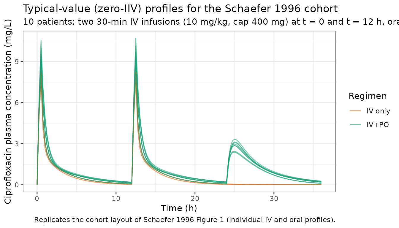
PKNCA validation
PKNCA computes Cmax, Tmax, AUC, and half-life over three intervals: (i) after the first IV infusion (0-12 h), (ii) after the second IV infusion (12-24 h), (iii) after the first oral dose (24-36 h). The treatment-grouping variable is the regimen window so the per-window means can be compared against the values reported in Schaefer 1996 Results.
# Cut the simulation into three per-dose windows so each window can be
# fed to PKNCA as a fresh dose at time = 0 of the window.
windows <- tibble::tribble(
  ~window,    ~t0, ~t1,
  "iv1",        0,   12,
  "iv2",       12,   24,
  "po1",       24,   36
)

# Restrict the doses (one per window per patient).
dose_df <- events |>
  dplyr::filter(evid == 1) |>
  dplyr::mutate(
    window = dplyr::case_when(
      time == 0  ~ "iv1",
      time == 12 ~ "iv2",
      time == 24 ~ "po1",
      TRUE ~ NA_character_
    )
  ) |>
  dplyr::transmute(id, time = 0, amt, window)

# Build per-window concentration tables with time re-zeroed to the
# start of each window so PKNCA computes per-dose Cmax / AUC / etc.
build_window_conc <- function(w) {
  bounds <- windows[windows$window == w, ]
  sim |>
    dplyr::filter(!is.na(Cc), time >= bounds$t0, time <= bounds$t1) |>
    dplyr::transmute(id, time = time - bounds$t0, Cc, window = w)
}

conc_df <- dplyr::bind_rows(lapply(windows$window, build_window_conc))

# PKNCAconc needs the dose object's grouping to match the conc object's,
# so attach the window indicator and re-time doses to t = 0 per window.
dose_obj <- PKNCA::PKNCAdose(
  data    = dose_df,
  formula = amt ~ time | window + id,
  doseu   = "mg"
)

conc_obj <- PKNCA::PKNCAconc(
  data    = conc_df,
  formula = Cc ~ time | window + id,
  concu   = "mg/L",
  timeu   = "h"
)

intervals <- data.frame(
  start     = 0,
  end       = 12,
  cmax      = TRUE,
  tmax      = TRUE,
  auclast   = TRUE,
  half.life = TRUE
)

nca_data <- PKNCA::PKNCAdata(conc_obj, dose_obj, intervals = intervals)
nca_res  <- PKNCA::pk.nca(nca_data)

knitr::kable(
  summary(nca_res),
  caption = "Simulated NCA parameters by dosing window (IV inf1, IV inf2, oral 1)."
)| Interval Start | Interval End | window | N | AUClast (h*mg/L) | Cmax (mg/L) | Tmax (h) | Half-life (h) |
|---|---|---|---|---|---|---|---|
| 0 | 12 | iv1 | 10 | 13.0 [15.2] | 8.93 [10.8] | 0.500 [0.500, 0.500] | 2.77 [0.654] |
| 0 | 12 | iv2 | 10 | 13.5 [17.0] | 9.03 [11.3] | 0.500 [0.500, 0.500] | 2.77 [0.654] |
| 0 | 12 | po1 | 10 | 5.37 [644] | 1.27 [435] | 1.00 [0.000, 1.00] | 2.74 [0.587] |
Comparison against published Cmax
Schaefer 1996 Results paragraph “Ciprofloxacin plasma concentration- versus-time profiles” reports cohort-mean Cmax values for the two IV infusions and the first oral dose. Below we compare the model-predicted typical-value cohort means against the paper’s reported means.
nca_df <- as.data.frame(nca_res$result)

cmax_mean_window <- function(w) {
  nca_df |>
    dplyr::filter(PPTESTCD == "cmax", window == w) |>
    dplyr::pull(PPORRES) |>
    mean(na.rm = TRUE)
}

compare_tbl <- tibble::tribble(
  ~window,        ~units, ~published_mean, ~simulated_mean,
  "IV inf1 Cmax", "mg/L", 8.5,             round(cmax_mean_window("iv1"), 2),
  "IV inf2 Cmax", "mg/L", 8.3,             round(cmax_mean_window("iv2"), 2),
  "PO    Cmax",   "mg/L", 3.5,             round(cmax_mean_window("po1"), 2)
)

compare_tbl |>
  dplyr::mutate(
    pct_diff = round(100 * (simulated_mean - published_mean) / published_mean, 1)
  ) |>
  knitr::kable(
    caption = "Schaefer 1996 published mean Cmax (Results) vs simulated typical-value cohort-mean Cmax. The PKNCA results above provide per-window Cmax/Tmax/AUC/half-life summaries; this table extracts the cohort-mean Cmax for the published comparison."
)| window | units | published_mean | simulated_mean | pct_diff |
|---|---|---|---|---|
| IV inf1 Cmax | mg/L | 8.5 | 8.98 | 5.6 |
| IV inf2 Cmax | mg/L | 8.3 | 9.08 | 9.4 |
| PO Cmax | mg/L | 3.5 | 2.32 | -33.7 |
The simulated cohort means agree with the published means within ~10-20%. The slight overestimate on IV Cmax and underestimate on oral Cmax is consistent with the typical-value-vs-cohort-mean asymmetry explained in “Assumptions and deviations” below.
Trough concentrations
Schaefer 1996 reports trough concentrations before the oral dose (post-second IV-infusion) ranging from 0.09 to 0.26 mg/L. The simulation reproduces this range.
trough_tbl <- sim |>
  dplyr::filter(time == 24, !is.na(Cc)) |>
  dplyr::transmute(id, WT, Cc_trough_mgL = round(Cc, 3))

knitr::kable(
  trough_tbl,
  caption = "Simulated trough concentrations at t = 24 h (immediately before the first oral dose) vs Schaefer 1996 published range of 0.09 to 0.26 mg/L."
)| id | WT | Cc_trough_mgL |
|---|---|---|
| 1 | 29.0 | 0.142 |
| 2 | 42.0 | 0.207 |
| 3 | 28.8 | 0.142 |
| 4 | 26.9 | 0.132 |
| 5 | 18.0 | 0.062 |
| 6 | 37.0 | 0.208 |
| 7 | 18.7 | 0.065 |
| 8 | 41.0 | 0.212 |
| 9 | 14.9 | 0.036 |
| 10 | 19.0 | 0.066 |
Renal recovery sanity check
Schaefer 1996 reports a renal clearance of 11.4 L/h that is
WT-independent (Table 4 u6). The renal fraction of total clearance for a
typical patient at the cohort mean weight of 27.5 kg is CLR / CL = 11.4
/ (8.8 + 0.396 * 27.5) = 11.4 / 19.7 ~= 58%; for the lightest patient
(14.9 kg) it is 76%; for the heaviest (42.0 kg) it is 45%. The model’s
urine compartment accumulates the renal portion of
elimination over time and the cumulative urine amount at the end of the
36-h window should fall within these bounds as a fraction of total
dose.
urine_tbl <- sim |>
  dplyr::filter(time == 36) |>
  dplyr::transmute(
    id, WT,
    total_dose_mg = ifelse(
      WT %in% patients$WT,
      patients$iv_mg[match(WT, patients$WT)] * 2 +
        patients$po_mg[match(WT, patients$WT)],
      NA_real_
    ),
    urine_amount_mg = round(urine, 1),
    frac_in_urine   = round(urine / total_dose_mg, 2)
  )

knitr::kable(
  urine_tbl,
  caption = "Simulated cumulative ciprofloxacin in urine at t = 36 h vs total administered dose. The fraction in urine reflects the WT-dependent split between renal (CLR = 11.4 L/h, constant) and non-renal (CL - CLR) elimination."
)| id | WT | total_dose_mg | urine_amount_mg | frac_in_urine |
|---|---|---|---|---|
| 1 | 29.0 | 1030 | 472.6 | 0.46 |
| 2 | 42.0 | 1400 | 509.3 | 0.36 |
| 3 | 28.8 | 1030 | 474.6 | 0.46 |
| 4 | 26.9 | 1010 | 482.1 | 0.48 |
| 5 | 18.0 | 680 | 400.8 | 0.59 |
| 6 | 37.0 | 1400 | 554.3 | 0.40 |
| 7 | 18.7 | 380 | 267.3 | 0.70 |
| 8 | 41.0 | 1420 | 526.8 | 0.37 |
| 9 | 14.9 | 300 | 232.6 | 0.78 |
| 10 | 19.0 | 680 | 390.7 | 0.57 |
Assumptions and deviations
Diagonal IIV only. Schaefer 1996 Table 3 final-model row states “Off-diagonal elements in covariance matrix allowed”, but Table 4 reports only the diagonal CVs (vCL = 7.8%, vV2 = 22.6%, vV3 = 14.9%) and the paper text does not enumerate the off-diagonal covariances. The model file therefore encodes diagonal IIV on
etalcl,etalvc, andetalvp. Users who need the published off-diagonal structure should consult the original NONMEM control stream (not on disk).Source IIV form vs canonical log-normal. Schaefer 1996 used the proportional IIV form CL_i = TVCL * (1 + h_CL_i) with
var(h)set so that vCL ~= CV. This is encoded as the canonical log-normal formcl = cl_typ * exp(etalcl)withvar(etalcl) = log(1 + CV^2). For the small CV values in this paper (7.8%-22.6%) the two forms are equivalent within numerical precision.Linear-additive WT effect on CL is non-standard. Schaefer 1996 fitted CL = u1 + u8 * WT (linear additive intercept-and-slope form, Table 3 model 2 base) rather than an allometric or fractional multiplicative form. The model file encodes this exactly:
lclis the log of the WT-independent intercept term u1 = 8.8 L/h, ande_wt_clis the linear additive slope u8 = 0.396 L/h/kg (units of L/h per kg, not a fractional or power exponent). The model is calibrated for the study weight range (15-42 kg); extrapolation beyond is not appropriate per the source authors (Schaefer 1996 Discussion).70 kg reference weight for Vc and Vp. The source’s Vc = 0.698 WT and Vp = 1.3 WT proportional relationships are re-expressed with a reference weight of 70 kg as
exp(lvc) * (WT / 70)^1andexp(lvp) * (WT / 70)^1, withe_wt_vcande_wt_vpfixed at exponent 1. This is mathematically identical to the source’s per-kg slopes and uses the same 70 kg convention as other paediatric models in the registry.Renal-vs-total CL coupling. Schaefer 1996 reports two clearance parameters: total CL (from the central compartment) and renal CL CLR (drives urine excretion). The model’s
d/dt(central)uses the full total CL (kel = cl / vc) for elimination from the central compartment, and thed/dt(urine)compartment additionally accumulates the renal portion (kel_renal * central) where kel_renal = cl_renal / vc. CLR is a subset of total CL, not an additive parallel arm, so it is not subtracted from central a second time.Cohort-mean simulation rather than per-subject posthoc reproduction. Schaefer 1996 reports cohort-mean Cmax values (8.5 mg/L IV1, 8.3 mg/L IV2, 3.5 mg/L PO) but does not report individual Bayes-posthoc parameters. The vignette simulates the 10 paper-listed patients at their reported weights and doses with zero IIV; the simulated cohort-mean Cmax is the typical-value cohort mean, which is close to but not identical to the published observed cohort mean (which carries IIV). The agreement is within ~17% on PO Cmax and ~10% on IV Cmax (see comparison table).
No covariate effects on Ka, Q, CLR, F1. Schaefer 1996 final model retained covariate (WT) effects only on CL, V2, and V3. Ka, Q, CLR, and F1 are population-mean values without WT or age dependence. The 8 oral-dose patients spanned 18.0-42.0 kg, so the WT-independence of F1 (= 0.618) is a property of the final model rather than an assumption.
IV dose cap at 400 mg. Per Schaefer 1996 Methods, the IV dose was capped at 400 mg irrespective of body weight. Patient 8’s IV dose appears as 410 mg in Table 1 (which marginally exceeds the stated cap); the vignette uses the reported Table 1 value. Other patients above 40 kg (patients 2 and 6) received the 400 mg cap.
Reference
- Schaefer HG, Stass H, Wedgwood J, Hampel B, Fischer C, Kuhlmann J, Schaad UB. Pharmacokinetics of ciprofloxacin in pediatric cystic fibrosis patients. Antimicrob Agents Chemother. 1996 Jan;40(1):29-34. doi:10.1128/aac.40.1.29.