Corifollitropin alfa (Zandvliet 2016) • nlmixr2lib

Model and source

Citation: Zandvliet AS, Prohn M, de Greef R, van Aarle F, McCrary Sisk C, Stegmann BJ. Impact of patient characteristics on the pharmacokinetics of corifollitropin alfa during controlled ovarian stimulation. Br J Clin Pharmacol. 2016;82(1):74-82. doi:10.1111/bcp.12939.
Article: https://doi.org/10.1111/bcp.12939

The packaged model is Zandvliet_2016_corifollitropin_alfa.

The model jointly describes corifollitropin alfa concentration (Cc, ng/mL) and total follicle stimulating hormone (FSH) immunoreactivity (FSHir, IU/L). Corifollitropin alfa is absorbed first-order from a subcutaneous depot into a one-compartment central pool with first-order elimination. An endogenous-FSH compartment carries the pre-dose steady-state baseline (FSHbaseline) and decays first-order at rate KeFSH after dosing (zero-order synthesis is set to zero from corifollitropin administration onwards, mirroring the paper’s structural model in the Methods / Structural model paragraph).

Population

Data from five phase II and III clinical trials of corifollitropin alfa in women undergoing controlled ovarian stimulation in a gonadotrophin- releasing hormone (GnRH) antagonist protocol followed by daily recombinant FSH from day 8 onwards. A total of 2630 women received 60-180 ug corifollitropin alfa SC; 2557 were evaluable for the population PK analysis. Cohort means by trial ranged 54.0 to 68.8 kg (body weight), 20.5 to 25.1 kg/m^2 (BMI), and 30.9 to 38.0 years (age); race composition was predominantly Caucasian with 1-45% Asian by trial (45.1% Asian in trial 107012, conducted in Korea and Taiwan) and 0.4-10% Black (Zandvliet 2016 Tables 1 and 2). The same information is available programmatically as readModelDb("Zandvliet_2016_corifollitropin_alfa")$population.

Source trace

Per-parameter origin is recorded as an in-file comment next to each ini() entry of inst/modeldb/specificDrugs/Zandvliet_2016_corifollitropin_alfa.R. The table below collects them in one place for review.

Equation / parameter	Value	Source location
`lka`	log(0.0436 1/h)	Table 3 theta_1
`lvc`	log(19.1 L)	Table 3 theta_2
`lcl`	log(0.19 L/h)	Table 3 theta_3
`lfdepot`	log(1) FIX	Table 3 theta_6
`e_wt_cl`	1.20	Table 3 theta_12
`e_wt_vc`	1.23	Table 3 theta_13
`e_bmi_fdepot`	-0.245	Table 3 theta_16
`e_race_asian_fdepot`	0.843	Table 3 theta_17
`e_race_black_fdepot`	1.13	Table 3 theta_18
`lkout` (KeFSH)	log(0.0101 1/h)	Table 3 theta_4
`lrbase` (FSHbaseline)	log(6.85 IU/L)	Table 3 theta_5
`e_age_kout`	-0.815	Table 3 theta_20
`e_race_asian_kout`	0.697	Table 3 theta_21
`e_wt_kout`	-0.832	Table 3 theta_22
`e_age_rbase`	0.423	Table 3 theta_19
`e_study_06029_fshir`	1.26	Table 3 theta_14
`e_study_38825_fshir`	1.12	Table 3 theta_15
`propSd` (Cc)	0.131	Table 3 theta_8
`propSd_FSHir`	0.0486	Table 3 theta_10
`addSd_FSHir`	0.717 IU/L	Table 3 theta_11
`etalka`	omega^2 = log(0.292^2 + 1)	Table 3 IIV row Ka (29.2% CV)
`etalcl + etalvc` (block)	(0.04764, 0.056, 0.08243)	Table 3 IIV rows CL/F (22.1% CV) and V/F (29.3% CV); covariance theta_* footnote
`etalkout`	omega^2 = log(0.29^2 + 1)	Table 3 IIV row KeFSH (29% CV; see Assumptions and deviations below)
`etalrbase`	omega^2 = log(0.267^2 + 1)	Table 3 IIV row FSHbaseline (26.7% CV)
`scale_fsh` (in `model()`)	6.11 IU/L per ng/mL FIX	Table 3 theta_7 (footnote ** “fixed to 6.11 as derived in a previous analysis”)
ODE: `d/dt(depot) = -ka*depot`	n/a	Methods / Structural model paragraph; Figure 3
ODE: `d/dt(central) = kadepot - kelcentral`	n/a	Methods / Structural model paragraph; Figure 3
ODE: `d/dt(endo_fsh) = -kout*endo_fsh` with `endo_fsh(0) = rbase`	n/a	Methods / Structural model paragraph (“Input of endogenous FSH was set to zero from administration of corifollitropin alfa onwards”)
Observable: `FSHir = (scale_fshCc + endo_fsh) 1.26^STUDY_06029 * 1.12^STUDY_38825`	n/a	Final-model paragraph and Table 3 theta_14 / theta_15

Virtual cohort

The published demographics inform a single typical-value cohort plus two sensitivity cohorts that exercise the body-weight and race covariates. Original observed data are not publicly available; the figures and NCA below use deterministic typical-value simulations (rxode2::zeroRe()) for direct comparison against the paper’s typical- value table, and a stochastic VPC for the time-course plot.

set.seed(20260620)

# Helper: per-subject covariate row plus a single SC dose at t = 0 and
# observation rows that exercise both observables (Cc and FSHir). All
# observation rows go to cmt = "Cc" -- both observables are
# algebraic in the model body, so rxode2 returns them as output columns
# regardless of which ODE state the observation row points at.
make_cohort <- function(n, wt, bmi, age, race_asian = 0L, race_black = 0L,
                        dose_ug = 150, id_offset = 0L, label) {
  obs_times <- seq(0, 192, by = 1)  # 8 days = 192 h, before rFSH starts
  subj <- tibble(
    id         = id_offset + seq_len(n),
    WT         = wt,
    BMI        = bmi,
    AGE        = age,
    RACE_ASIAN = race_asian,
    RACE_BLACK = race_black,
    STUDY_06029 = 0L,
    STUDY_38825 = 0L,
    cohort     = label
  )
  doses <- subj |>
    mutate(time = 0, amt = dose_ug, evid = 1L, cmt = "depot")
  obs <- subj |>
    tidyr::crossing(time = obs_times) |>
    mutate(amt = NA_real_, evid = 0L, cmt = "Cc")
  bind_rows(doses, obs) |>
    arrange(id, time, evid)
}

# Cohort A: typical Caucasian subject from the paper's typical-value
# calculation (67.1 kg, BMI 24.6 kg/m^2, 32 years; dose 150 ug because
# WT > 60 kg). The paper reports for this subject Cmax = 4.43 ng/mL,
# tmax = 43.9 h, AUC_inf = 688 ng h/mL, t-half = 69.4 h.
# Cohort B: lower-weight Caucasian subject (54 kg, BMI 20.5 kg/m^2 from
# trial 107012 Table 2) on the WT <= 60 kg dose level of 100 ug.
# Cohort C: typical Asian subject (54 kg, BMI 20.5 kg/m^2) on 100 ug
# to demonstrate the race-on-bioavailability effect.
events <- bind_rows(
  make_cohort(n = 50,  wt = 67.1, bmi = 24.6, age = 32, race_asian = 0L,
              race_black = 0L, dose_ug = 150, id_offset =   0L,
              label = "Caucasian, 67.1 kg, 150 ug"),
  make_cohort(n = 50,  wt = 54.0, bmi = 20.5, age = 32, race_asian = 0L,
              race_black = 0L, dose_ug = 100, id_offset = 100L,
              label = "Caucasian, 54 kg, 100 ug"),
  make_cohort(n = 50,  wt = 54.0, bmi = 20.5, age = 32, race_asian = 1L,
              race_black = 0L, dose_ug = 100, id_offset = 200L,
              label = "Asian, 54 kg, 100 ug")
)
stopifnot(!anyDuplicated(unique(events[, c("id", "time", "evid")])))

Simulation

mod <- readModelDb("Zandvliet_2016_corifollitropin_alfa")

# Stochastic VPC for the time-course plot. `` keeps
# rxode2 from auto-converting the ODE system to its linear-compartment
# fast path, which silently breaks the multi-output dvid->cmt mapping
# for models with two algebraic observables on different ODE-state
# subsets (see known-vignette-failure-patterns.md pattern 5b).
sim_vpc <- rxode2::rxSolve(
  mod,
  events = events,
  keep       = c("cohort", "WT", "BMI", "AGE", "RACE_ASIAN")
) |> as.data.frame()

For deterministic typical-value comparison against the paper’s typical-subject Cmax / tmax / AUC / half-life, zero out the random effects.

mod_typical <- rxode2::zeroRe(mod)
events_typical <- events |>
  group_by(cohort) |>
  filter(id == min(id)) |>
  ungroup()
sim_typical <- rxode2::rxSolve(
  mod_typical,
  events    = events_typical,
  keep      = c("cohort", "WT", "BMI", "AGE", "RACE_ASIAN")
) |> as.data.frame()
#> ℹ omega/sigma items treated as zero: 'etalcl', 'etalvc', 'etalka', 'etalkout', 'etalrbase'
#> Warning: multi-subject simulation without without 'omega'

Replicate published figures

# Stochastic VPC of corifollitropin alfa concentration vs time.
# Replicates the panel-A shape of Figure 4 (trial 107012 VPC for
# corifollitropin alfa levels) at the cohort-level summary.
sim_vpc |>
  group_by(time, cohort) |>
  summarise(
    Q05 = quantile(Cc, 0.05, na.rm = TRUE),
    Q50 = quantile(Cc, 0.50, na.rm = TRUE),
    Q95 = quantile(Cc, 0.95, na.rm = TRUE),
    .groups = "drop"
  ) |>
  ggplot(aes(time, Q50)) +
  geom_ribbon(aes(ymin = Q05, ymax = Q95), alpha = 0.25) +
  geom_line() +
  facet_wrap(~cohort) +
  labs(x = "Time (h)", y = "Corifollitropin alfa (ng/mL)",
       title = "Cc time course by cohort",
       caption = "5/50/95% summary across 50 virtual subjects per cohort. Replicates the shape of Figure 4 panel A of Zandvliet 2016 (trial 107012 corifollitropin alfa VPC).")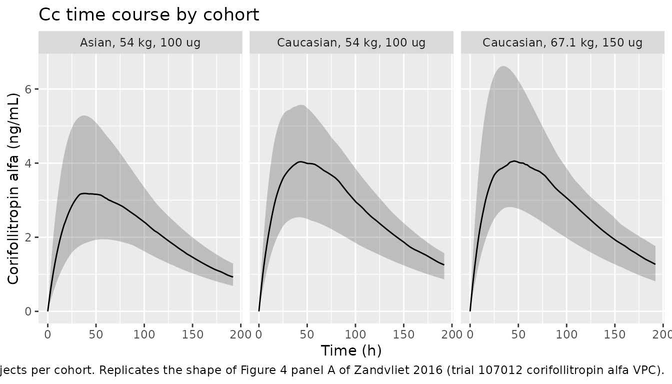

# Stochastic VPC of total FSH immunoreactivity vs time.
# Replicates the panel-B shape of Figure 4 (trial 107012 VPC for
# total FSH immunoreactivity).
sim_vpc |>
  group_by(time, cohort) |>
  summarise(
    Q05 = quantile(FSHir, 0.05, na.rm = TRUE),
    Q50 = quantile(FSHir, 0.50, na.rm = TRUE),
    Q95 = quantile(FSHir, 0.95, na.rm = TRUE),
    .groups = "drop"
  ) |>
  ggplot(aes(time, Q50)) +
  geom_ribbon(aes(ymin = Q05, ymax = Q95), alpha = 0.25) +
  geom_line() +
  facet_wrap(~cohort) +
  labs(x = "Time (h)", y = "Total FSH immunoreactivity (IU/L)",
       title = "FSHir time course by cohort",
       caption = "5/50/95% summary across 50 virtual subjects per cohort. Replicates the shape of Figure 4 panel B of Zandvliet 2016 (trial 107012 total FSH immunoreactivity VPC).")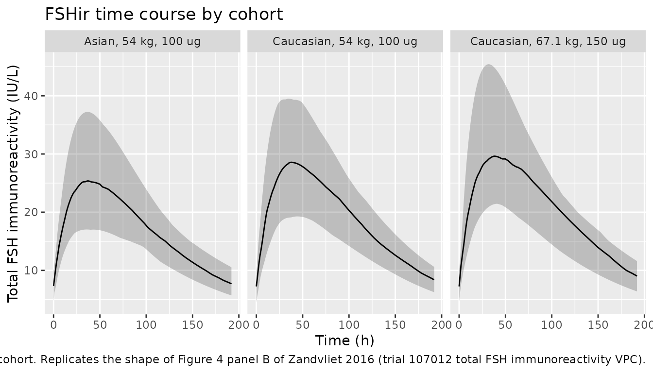

PKNCA validation

# Cc per-subject concentrations for NCA. Use only the typical-value
# simulation; PKNCA on a single trajectory per cohort directly
# reproduces the paper's typical-value PK parameter calculation.
sim_nca <- sim_typical |>
  dplyr::filter(!is.na(Cc)) |>
  dplyr::select(id, time, Cc, cohort)

# Guarantee a time = 0 row per (id, cohort); pre-dose extravascular
# Cc = 0 is the correct value. (See pknca-recipes.md "Time-zero
# guarantee".)
sim_nca <- bind_rows(
  sim_nca,
  sim_nca |> distinct(id, cohort) |> mutate(time = 0, Cc = 0)
) |>
  distinct(id, cohort, time, .keep_all = TRUE) |>
  arrange(id, cohort, time)

conc_obj <- PKNCA::PKNCAconc(sim_nca, Cc ~ time | cohort + id)

dose_df <- events_typical |>
  dplyr::filter(evid == 1L) |>
  dplyr::select(id, time, amt, cohort)
dose_obj <- PKNCA::PKNCAdose(dose_df, amt ~ time | cohort + id)

intervals <- data.frame(
  start       = 0,
  end         = Inf,
  cmax        = TRUE,
  tmax        = TRUE,
  aucinf.obs  = TRUE,
  half.life   = TRUE
)

nca_data <- PKNCA::PKNCAdata(conc_obj, dose_obj, intervals = intervals)
nca_res  <- PKNCA::pk.nca(nca_data)

Comparison against published NCA

The paper reports for the typical Caucasian subject (67.1 kg, BMI 24.6 kg/m^2) a single set of typical-value NCA-style PK descriptors (Results / Final model paragraph):

Cmax = 4.43 ng/mL at tmax = 43.9 h
AUC = 688 ng h/mL
Terminal half-life = 69.4 h

published <- tibble::tribble(
  ~cohort,                      ~cmax,  ~tmax, ~aucinf.obs, ~half.life,
  "Caucasian, 67.1 kg, 150 ug",  4.43,  43.9,   688.0,        69.4
)

cmp <- nlmixr2lib::ncaComparisonTable(
  simulated     = nca_res,
  reference     = published,
  by            = "cohort",
  units         = c(cmax = "ng/mL", aucinf.obs = "ng*h/mL",
                    tmax = "h", half.life = "h"),
  tolerance_pct = 20
)

knitr::kable(
  cmp,
  caption = "Simulated typical-value vs. Zandvliet 2016 published typical-value NCA-style PK parameters for the reference Caucasian subject. * differs from reference by >20%.",
  align   = c("l", "l", "r", "r", "r")
)

Simulated typical-value vs. Zandvliet 2016 published typical-value NCA-style PK parameters for the reference Caucasian subject. * differs from reference by >20%.
NCA parameter	cohort	Reference	Simulated	% diff
Cmax (ng/mL)	Caucasian, 67.1 kg, 150 ug	4.43	4.37	-1.4%
Tmax (h)	Caucasian, 67.1 kg, 150 ug	43.9	44	+0.2%
AUC0-∞ (obs) (ng*h/mL)	Caucasian, 67.1 kg, 150 ug	688	685	-0.5%
t½ (h)	Caucasian, 67.1 kg, 150 ug	69.4	71.8	+3.5%

The 54 kg cohorts have no per-subject published Cmax / AUC reference; they are included to exercise the model’s body-weight and race covariates rather than for direct comparison.

Body-weight effect on dose-normalised exposure

The paper reports that “in subjects with a similar BMI of 24 kg/m^2, body weight would contribute to an increase in corifollitropin alfa dose-normalised exposure of approximately 89% in women with a body weight of 50 kg compared with women with a body weight of 90 kg treated with the same dose” (Results / Body weight and BMI paragraph). The deterministic typical-value AUC across a body-weight grid at the fixed BMI of 24 kg/m^2 should reproduce this approximately-89% effect.

wt_grid <- c(50, 60, 70, 80, 90)
events_wt <- bind_rows(
  lapply(seq_along(wt_grid), function(i) {
    make_cohort(n = 1L, wt = wt_grid[i], bmi = 24,
                age = 32, race_asian = 0L, race_black = 0L,
                dose_ug = 100, id_offset = 1000L + 100L * i,
                label = sprintf("%g kg", wt_grid[i]))
  })
)
sim_wt <- rxode2::rxSolve(
  rxode2::zeroRe(mod),
  events    = events_wt,
  keep      = c("cohort", "WT")
) |> as.data.frame()
#> ℹ omega/sigma items treated as zero: 'etalcl', 'etalvc', 'etalka', 'etalkout', 'etalrbase'
#> Warning: multi-subject simulation without without 'omega'

sim_wt_nca <- sim_wt |>
  dplyr::filter(!is.na(Cc)) |>
  dplyr::select(id, time, Cc, cohort)
sim_wt_nca <- bind_rows(
  sim_wt_nca,
  sim_wt_nca |> distinct(id, cohort) |> mutate(time = 0, Cc = 0)
) |>
  distinct(id, cohort, time, .keep_all = TRUE) |>
  arrange(id, cohort, time)

conc_wt <- PKNCA::PKNCAconc(sim_wt_nca, Cc ~ time | cohort + id)
dose_wt <- PKNCA::PKNCAdose(
  events_wt |> filter(evid == 1L) |> select(id, time, amt, cohort),
  amt ~ time | cohort + id
)
nca_wt <- PKNCA::pk.nca(
  PKNCA::PKNCAdata(conc_wt, dose_wt,
                   intervals = data.frame(start = 0, end = Inf,
                                          aucinf.obs = TRUE))
)
auc_wt <- as.data.frame(nca_wt$result) |>
  filter(PPTESTCD == "aucinf.obs") |>
  transmute(WT = as.numeric(sub(" kg", "", cohort)),
            AUCinf = PPORRES)

auc_50 <- auc_wt$AUCinf[auc_wt$WT == 50]
auc_90 <- auc_wt$AUCinf[auc_wt$WT == 90]
ratio_50_90 <- auc_50 / auc_90

knitr::kable(
  auc_wt,
  digits = 1,
  caption = sprintf(
    "Dose-normalised typical-value AUC at fixed BMI = 24 kg/m^2 and dose 100 ug. The 50 kg / 90 kg AUC ratio is %.2f, i.e., %.0f%% higher exposure at 50 kg (paper text: ~89%% higher).",
    ratio_50_90, 100 * (ratio_50_90 - 1)
  )
)

Dose-normalised typical-value AUC at fixed BMI = 24 kg/m^2 and dose 100 ug. The 50 kg / 90 kg AUC ratio is 2.02, i.e., 102% higher exposure at 50 kg (paper text: ~89% higher).
WT	AUCinf
50	653.5
60	525.1
70	436.4
80	371.8
90	322.8

Assumptions and deviations

The Ke_FSH inter-individual variability is reported as a 29% CV in Zandvliet 2016 Table 3 with a 95% bootstrap CI of 51.4-69.7% that does not bracket the point estimate. The published table cell is internally inconsistent; an alternative reading where the cell value represents omega^2 = 0.29 gives a CV of approximately 58% which would be consistent with the printed CI. The model file uses the face-value 29% CV (omega^2 = log(0.29^2 + 1) = 0.08074) on the KeFSH eta. The IIV on KeFSH affects only the endogenous-FSH submodel decay rate and does not appear in the typical-value Cmax / AUC / half-life comparison above. If a future operator recovers the original NONMEM .lst file or an author correction, update the model file accordingly.
The scaling factor SCALE = 6.11 IU/L per ng/mL is a fixed assay- conversion factor inherited from an upstream analysis cited in Zandvliet 2016 Table 3 (theta_7 footnote: “scaling factor fixed to 6.11 as derived in a previous analysis”). Encoded as the constant scale_fsh in the model() block rather than as a fixed ini() parameter because it is not part of this paper’s structural fit.
The two trial-specific multiplicative effects on the FSH immunoreactivity observation (1.26 for trial 06029 and 1.12 for trial 38825) are exposed via binary covariates STUDY_06029 and STUDY_38825 that default to 0 for general simulation use. To reproduce one of those two trials’ FSH immunoreactivity prediction, set the matching indicator to 1 on the relevant subjects.
The exponents on body weight, BMI, and age in the covariate- relationship column of Table 3 are read with the sign implied by the 95% CI brackets (e_bmi_fdepot = -0.245, e_age_kout = -0.815, e_wt_kout = -0.832). The signs are confirmed independently by the paper text: higher BMI lowers dose-normalised exposure (Results / Body weight and BMI paragraph), so the BMI effect on F is negative; the 95% CIs -1.206, -0.425 and -1.37, -0.23 bracket the AGE and WT exponents on KeFSH in the negative half-line.
Dose units are micrograms (ug) and apparent volume is in litres (L). Cc = central / vc therefore has units ug/L = ng/mL directly with no conversion factor required.
The race-effect parameters e_race_asian_fdepot = 0.843, e_race_black_fdepot = 1.13, and e_race_asian_kout = 0.697 enter the model as power-of-indicator factors (X^RACE_ASIAN, X^RACE_BLACK) so that the effect collapses to 1 when the indicator is 0 and to X when the indicator is 1. This reproduces the published theta_17^ASIAN and theta_18^BLACK and theta_21^ASIAN source-paper forms in Table 3.
The endogenous FSH submodel encodes only the post-dose decay behaviour the paper actually fits: zero-order synthesis of endogenous FSH is set to zero from corifollitropin alfa administration onwards (Methods / Structural model). The steady-state baseline FSHbaseline (rbase) is loaded directly as endo_fsh(0) <- rbase. Pre-dose simulations that need the steady-state hold are achieved by an evid = 0 observation at t = 0 with no dose: the compartment starts at rbase and decays only after a corifollitropin alfa dose is administered.
The endogenous-FSH compartment is named endo_fsh and is declared as a paper_specific_compartments because the compartment role (endogenous-hormone baseline pool with elimination-only kinetics post-dose) is paper-mechanistic and does not match any canonical nlmixr2lib compartment role.