Vancomycin in critically ill children, cystatin C (Downes 2020)
Source:vignettes/articles/Downes_2020_vancomycin.Rmd
Downes_2020_vancomycin.RmdModel and source
Downes 2020 fitted a one-compartment population PK model for intravenous vancomycin in 20 critically ill children and compared seven estimated-GFR equations as the renal covariate on clearance. The combined creatinine-cystatin C full age spectrum equation (FAScomb) fitted best, and female sex lowered clearance further.
mod <- readModelDb("Downes_2020_vancomycin")
ui <- rxode2::rxode(mod)
#> ℹ parameter labels from comments will be replaced by 'label()'- Citation: Downes KJ, Zane NR, Zuppa AF. Effect of Cystatin C on Vancomycin Clearance Estimation in Critically Ill Children Using a Population Pharmacokinetic Modeling Approach. Ther Drug Monit. 2020;42(6):848-855. doi:10.1097/FTD.0000000000000796. Preliminary results presented as Downes K, Zuppa A. Cystatin C Improves Estimation of Vancomycin Clearance in Critically Ill Children Using a Population Pharmacokinetic Modeling Approach. Open Forum Infect Dis. 2018;5(Suppl 1):S431 (IDWeek 2018 abstract 1402).
- Article: https://doi.org/10.1097/FTD.0000000000000796 (author manuscript PMC7669697)
- Supplement: Supplemental Figure 1 (observed concentrations) and Supplemental Figure 2 (Monte Carlo profiles) only; there is no control stream.
The same cohort was first reported as IDWeek 2018 abstract 1402 (Open Forum Infect Dis 2018;5(Suppl 1):S431). That abstract describes a different model – two-compartment, normalized to 70 kg, with no sex effect – and reports no peripheral volume, exponents, variability or residual error. The packaged model is the final model of the full 2020 paper, which replaced the abstract’s structure with a one-compartment model.
Population
Twenty children aged 2-18 years receiving IV vancomycin in the PICU of the Children’s Hospital of Philadelphia, December 2015 to November 2017 (Downes 2020 Table 2): median age 12.7 years (IQR 8.8-15.5, range 3.9-18.2), weight 33.9 kg (IQR 25.9-45.9), 6 of 20 female, 55% mechanically ventilated, 40% on steroids. Initial dosing was a median 54.8 mg/kg/day (IQR 37.4-59.4), every 6 h in 70% of children. FAScomb eGFR at PK sampling was a median 145 mL/min/1.73 m^2 (IQR 109-175): renal function was largely normal or augmented. The 20 children contributed 83 concentrations, 58 from one steady-state dosing interval (1 h and 3.5 h after the end of the infusion and a pre-dose trough) and 25 from clinical care.
str(ui$population, max.level = 1, give.attr = FALSE)
#> List of 14
#>  $ species         : chr "human"
#>  $ n_subjects      : int 20
#>  $ n_studies       : int 1
#>  $ n_sites         : int 1
#>  $ n_concentrations: int 83
#>  $ age_range       : chr "3.9-18.2 years (eligibility 2-18 years)"
#>  $ age_median      : chr "12.7 years (IQR 8.8-15.5)"
#>  $ weight_median   : chr "33.9 kg (IQR 25.9-45.9)"
#>  $ sex_female_pct  : num 30
#>  $ disease_state   : chr "Critically ill children in the PICU receiving intravenous vancomycin for any indication (sepsis or rule-out sep"| __truncated__
#>  $ dose_range      : chr "Clinician-chosen intermittent IV regimens, typically 10-15 mg/kg every 6-8 h infused over 1-2 h; initial dosing"| __truncated__
#>  $ regions         : chr "United States (Children's Hospital of Philadelphia)"
#>  $ renal_function  : chr "FAScomb eGFR median 145 mL/min/1.73 m^2 (IQR 109-175) and bedside Schwartz eGFR median 138 (IQR 97-179) at PK s"| __truncated__
#>  $ notes           : chr "Prospective observational study, December 2015 to November 2017. 83 vancomycin concentrations (58 research samp"| __truncated__
Source trace
Per-parameter origin is recorded beside each ini()
entry; collected here.
| Parameter | Value | Source |
|---|---|---|
lcl |
log(4.02 L/h) | Table 4, CL (typical 34-kg male, eGFR 145) |
lvc |
log(16.4 L) | Table 4, V |
e_wt_cl |
0.75, fixed | Results (estimated 0.74, then fixed at 0.75); Table 4 footnote a |
e_wt_vc |
1, fixed | Methods (“V_d was scaled to 1”); Table 4 footnote a |
e_crcl_cl |
0.903 | Table 4, eGFR from FAScomb |
e_sexf_cl |
0.699 | Table 4, Female sex; footnote a “(0.699 if female)” |
etalcl |
0.234^2 = 0.054756 | Table 4, IIV clearance 23.4; footnote b (CV = sqrt(variance) x 100) |
| IIV on V | not estimated | Table 4 prints NA |
propSd |
0.179 | Table 4, residual proportional; footnote c (reported as SD) |
addSd |
2.44 mg/L | Table 4, residual additive (read as SD; see Assumptions) |
| Reference weight 34 kg, eGFR 145 | – | Table 4 footnote a |
Final model equations (Table 4 footnote a):
CL (L/hr) = 4.02 * (WT/34)^0.75 * (eGFR/145)^0.903 * (0.699 if female)
V  (L)    = 16.4 * (WT/34)
Verification 1: transcription against a hand-typed closed form
A one-compartment model receiving a constant-rate infusion at steady state has a closed-form solution. The function below is written only from the printed constants, independently of the model file, so a transcription error in the model file makes the two disagree.
# Steady-state concentration, one compartment, infusion of `dose` over `tinf`
# repeated every `tau`; t is time since the start of the current infusion.
cf_ss <- function(t, dose, tinf, tau, cl, v) {
  k <- cl / v
  r0 <- dose / tinf
  acc <- 1 / (1 - exp(-k * tau))
  ifelse(
    t <= tinf,
    r0 / cl * ((1 - exp(-k * t)) + (1 - exp(-k * tinf)) * exp(-k * (t + tau - tinf)) * acc),
    r0 / cl * (1 - exp(-k * tinf)) * exp(-k * (t - tinf)) * acc
  )
}

# Typed directly from Downes 2020 Table 4 footnote a.
hand_params <- function(WT, CRCL, SEXF) {
  list(
    cl = 4.02 * (WT / 34)^0.75 * (CRCL / 145)^0.903 * ifelse(SEXF == 1, 0.699, 1),
    v = 16.4 * (WT / 34)
  )
}
TAU <- 6
TINF <- 1
gate_grid <- sort(unique(c(seq(0, TAU, by = 0.02), TINF)))
mod_typical <- rxode2::zeroRe(mod)
#> ℹ parameter labels from comments will be replaced by 'label()'

gate_points <- tibble::tribble(
  ~point,                         ~WT, ~CRCL, ~SEXF,
  "reference subject (male)",     34,  145,   0,
  "off-reference subject (female)", 18, 90,   1
)

gate <- lapply(seq_len(nrow(gate_points)), function(i) {
  gp <- gate_points[i, ]
  dose <- 15 * gp$WT
  ev <- rbind(
    data.frame(time = 0, amt = dose, evid = 1L, cmt = "central", ii = TAU, ss = 1L, dur = TINF),
    data.frame(time = gate_grid, amt = NA_real_, evid = 0L, cmt = "central", ii = 0, ss = 0L, dur = 0)
  )
  ev$id <- 1L
  ev$WT <- gp$WT
  ev$CRCL <- gp$CRCL
  ev$SEXF <- gp$SEXF
  s <- as.data.frame(rxode2::rxSolve(mod_typical, events = ev, returnType = "data.frame",
                                     rtol = 1e-10, atol = 1e-12))
  p <- hand_params(gp$WT, gp$CRCL, gp$SEXF)
  ref <- cf_ss(s$time, dose, TINF, TAU, p$cl, p$v)
  tibble(Point = gp$point, `CL (L/h)` = p$cl, `V (L)` = p$v,
         max_rel_err = max(abs(s$Cc - ref) / ref))
}) |> bind_rows()
#> ℹ omega/sigma items treated as zero: 'etalcl'
#> ℹ omega/sigma items treated as zero: 'etalcl'

gate |>
  mutate(`Max relative error` = format(max_rel_err, digits = 2, scientific = TRUE)) |>
  select(-max_rel_err) |>
knitr::kable(digits = 3, caption = "Packaged model vs. an independent closed form built from the printed constants.")| Point | CL (L/h) | V (L) | Max relative error |
|---|---|---|---|
| reference subject (male) | 4.020 | 16.400 | 9.4e-08 |
| off-reference subject (female) | 1.134 | 8.682 | 7.5e-07 |
# Pure numerical error between a solve and its own closed form, with the same
# parameters on both sides: a tight bound is correct and machine-stable.
stopifnot(nrow(gate) == 2, all(is.finite(gate$max_rel_err)), max(gate$max_rel_err) < 1e-6)
stopifnot(abs(gate$`CL (L/h)`[1] - 4.02) < 1e-12)
The reference subject recovers the printed 4.02 L/h exactly, and the off-reference female subject exercises every exponent, both reference constants and the sex factor.
Virtual cohort
Individual data are not public. The cohort reproduces the Table 2 quantiles: weight and FAScomb eGFR are drawn log-normally with the median as location and the interquartile range setting the scale, and 30% are female.
# set.seed() seeds R's RNG only; rxode2's own streams differ across thread
# counts, so the assertions below are written on the centre of the
# distribution, not its extremes.
set.seed(20201201)
N <- 200L # validation cohorts are capped at 200 per arm

lnq <- function(n, med, q1, q3) {
  stats::rlnorm(n, meanlog = log(med), sdlog = log(q3 / q1) / (2 * stats::qnorm(0.75)))
}

subj <- tibble(
  id = seq_len(N),
  WT = pmin(pmax(lnq(N, 33.9, 25.9, 45.9), 12), 110), # Table 2 weight; clipped to a plausible 4-18 y range
  CRCL = lnq(N, 145, 109, 175),                        # Table 2 FAScomb eGFR at PK sampling
  SEXF = stats::rbinom(N, 1, 0.30)                     # Table 2: 6 of 20 female
)
Simulation: the paper’s Monte Carlo regimen
Downes 2020 (Methods, Simulations) simulated 15 mg/kg every 6 hours for the study cohort and reported a median simulated trough at 36 h of 12.8 mg/L for the FAScomb model (Results). The same regimen is used here with a 1-hour infusion (the paper’s institutional range was 1-2 h; the simulation duration is not stated).
DOSE_MGKG <- 15
dose_times <- seq(0, 42, by = TAU)
obs_grid <- sort(unique(c(seq(0, 48, by = 0.25), dose_times + TINF)))

events <- bind_rows(
  subj |>
    tidyr::expand_grid(time = dose_times) |>
    mutate(amt = DOSE_MGKG * WT, evid = 1L, dur = TINF),
  subj |>
    tidyr::expand_grid(time = obs_grid) |>
    mutate(amt = NA_real_, evid = 0L, dur = 0)
) |>
  mutate(cmt = "central", treatment = "15 mg/kg q6h") |>
  arrange(id, time, desc(evid))

sim <- as.data.frame(rxode2::rxSolve(mod, events = events, keep = c("WT", "CRCL", "SEXF", "treatment"),
                                     returnType = "data.frame"))
#> ℹ parameter labels from comments will be replaced by 'label()'
stopifnot(nrow(sim) > 0, !anyNA(sim$Cc), all(sim$Cc >= 0))
sim |>
  group_by(time) |>
  summarise(Q05 = quantile(Cc, 0.05), Q50 = median(Cc), Q95 = quantile(Cc, 0.95), .groups = "drop") |>
  ggplot(aes(time, Q50)) +
  geom_ribbon(aes(ymin = Q05, ymax = Q95), alpha = 0.25, fill = "steelblue") +
  geom_line(linewidth = 0.7) +
  geom_hline(yintercept = c(10, 20), linetype = "dashed", colour = "grey40") +
  geom_vline(xintercept = 36, linetype = "dotted") +
  labs(x = "Time (h)", y = "Vancomycin (mg/L)",
       caption = paste("Median and 90% prediction interval (individual predictions) across 200 virtual",
                       "children at 15 mg/kg q6h. Dashed: the 10-20 mg/L trough target used",
                       "clinically (Methods). Dotted: the 36-h trough reported in the paper.",
                       "Compare with Supplemental Figure 2 of Downes 2020 (red curves)."))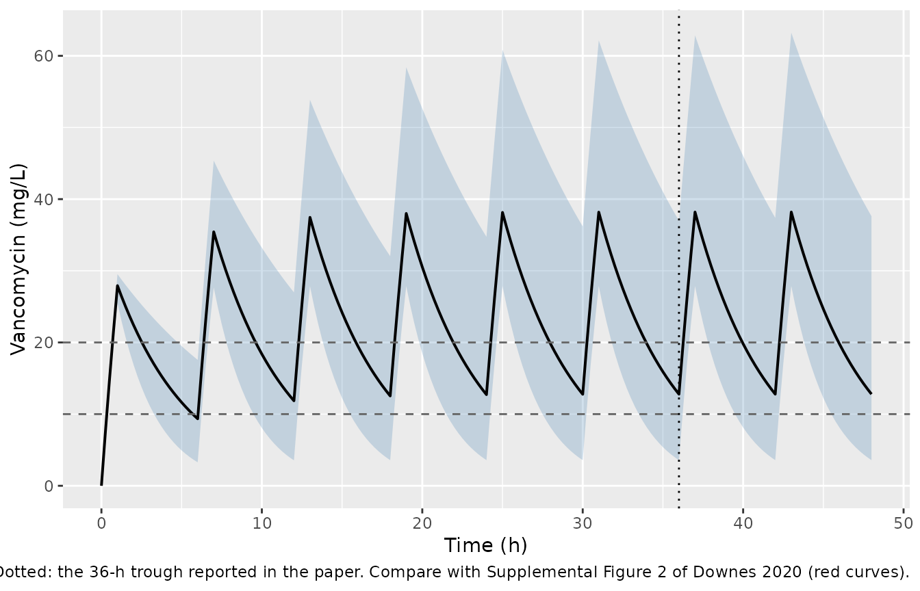
Comparison against the published simulated trough
trough36 <- sim |> filter(time == 36)
stopifnot(nrow(trough36) == N)
tr <- tibble(
  Quantity = c("Median Cc at 36 h, individual prediction", "Median at 36 h, with residual error"),
  Simulated = c(median(trough36$Cc), median(trough36$sim)),
  Published = 12.8
) |>
  mutate(`Difference (%)` = 100 * (Simulated / Published - 1))
knitr::kable(tr, digits = 2, caption = "Median simulated trough at 36 h, 15 mg/kg q6h (Downes 2020 Results: 12.8 mg/L).")| Quantity | Simulated | Published | Difference (%) |
|---|---|---|---|
| Median Cc at 36 h, individual prediction | 12.78 | 12.8 | -0.15 |
| Median at 36 h, with residual error | 12.33 | 12.8 | -3.70 |
PKNCA validation
The dose given at 36 h starts the dosing interval whose pre-dose
concentration is the paper’s 36-h trough. Because accumulation from the
first dose is monotone, cmin over 36-42 h is that pre-dose
trough.
# Only `!is.na(Cc)`: a `time > 0` or `Cc > 0` filter would drop the time-zero
# record PKNCA needs.
sim_nca <- sim |>
  filter(!is.na(Cc)) |>
  select(id, time, Cc, treatment)
stopifnot(all(tapply(sim_nca$time, sim_nca$id, min) == 0))

conc_obj <- PKNCA::PKNCAconc(sim_nca, Cc ~ time | treatment + id, concu = "mg/L", timeu = "h")
dose_obj <- PKNCA::PKNCAdose(
  events |> filter(evid == 1L) |> select(id, time, amt, treatment),
  amt ~ time | treatment + id, doseu = "mg"
)
intervals <- data.frame(start = 36, end = 42, cmax = TRUE, tmax = TRUE, cmin = TRUE,
                        auclast = TRUE, cav = TRUE)
nca_res <- PKNCA::pk.nca(PKNCA::PKNCAdata(conc_obj, dose_obj, intervals = intervals))
nca_tbl <- as.data.frame(nca_res$result)
stopifnot(nrow(nca_tbl) > 0, all(c("cmin", "auclast") %in% nca_tbl$PPTESTCD))
published <- tibble::tribble(
  ~treatment,      ~cmin,
  "15 mg/kg q6h",  12.8 # Downes 2020 Results: median simulated Cmin at 36 h (FAScomb model)
)
cmp <- nlmixr2lib::ncaComparisonTable(
  simulated = nca_res,
  reference = published,
  by = "treatment",
  params = "cmin",
  units = c(cmin = "mg/L"),
  tolerance_pct = 20
)
knitr::kable(cmp, caption = "Simulated vs. published median trough at 36 h. * differs by more than 20%.")| NCA parameter | treatment | Reference | Simulated | % diff |
|---|---|---|---|---|
| Cmin (mg/L) | 15 mg/kg q6h | 12.8 | 12.8 | -0.1% |
nca_tbl |>
  filter(PPTESTCD %in% c("cmax", "cmin", "auclast", "cav")) |>
  group_by(PPTESTCD) |>
  summarise(Median = median(PPORRES), `5th` = quantile(PPORRES, 0.05),
            `95th` = quantile(PPORRES, 0.95), .groups = "drop") |>
  mutate(Parameter = nlmixr2lib::ncaParamLabel(
    PPTESTCD, units = c(cmax = "mg/L", cmin = "mg/L", auclast = "mg*h/L", cav = "mg/L")
  )) |>
  select(Parameter, Median, `5th`, `95th`) |>
  knitr::kable(digits = 2, caption = paste(
    "Exposures over the 36-42 h dosing interval at 15 mg/kg q6h. Only the trough",
"is reported by the paper; the rest are predictions."))| Parameter | Median | 5th | 95th |
|---|---|---|---|
| AUClast (mg*h/L) | 142.01 | 75.67 | 295.24 |
| Cavg (mg/L) | 23.67 | 12.61 | 49.21 |
| Cmax (mg/L) | 38.20 | 27.87 | 62.86 |
| Cmin (mg/L) | 12.78 | 3.58 | 36.97 |
Over 24 h near steady state the AUC is roughly four times the 6-h interval AUC above. The Discussion’s target of AUC 400-600 mg*h/L is the context for the authors’ statement that most children need 60-80 mg/kg/day.
Assumptions and deviations
-
Additive residual read as an SD. Table 4 prints the
additive residual as
2.44with no units and no footnote, while the proportional row carries footnote c (“reported as standard deviation”). Following a maintainer ruling, 2.44 is read as an SD in mg/L (addSd = 2.44). The alternative reading, a raw NONMEM SIGMA variance, would giveaddSd = sqrt(2.44) = 1.562 mg/L. The term has an RSE of 106%, so it is weakly identified either way. The choice affects stochastic simulations and Bayesian reuse, not typical-value predictions. -
Residual combination. “Additive plus proportional”
is encoded with nlmixr2’s default combined form (variances add),
matching NONMEM’s
Y = F*(1 + EPS1) + EPS2. -
IIV on clearance. Footnote b defines the reported
23.4 as sqrt(variance) x 100, so
omega^2 = 0.234^2. IIV on volume is NA in Table 4 and is not included. -
The eGFR covariate needs the FAS Q_Cr table.
FAScomb (Table 1) is
107.3 / [(Cr/Q_Cr + CysC/Q_CysC) / 2]withQ_CysC = 0.82 mg/LandQ_Crthe age-specific normal creatinine from the FAS publication (Pottel et al.), which Downes 2020 does not reproduce. Users must computeCRCLfrom that source; the virtual cohort here samples eGFR directly from its Table 2 quantiles instead. - Virtual cohort. Weight, eGFR and sex are drawn independently from the Table 2 summary statistics; the paper’s Monte Carlo used the 20 subjects’ actual baseline characteristics, whose joint distribution is not published. The paper simulated with baseline eGFR, whose FAScomb median is not reported, so the PK-sampling eGFR quantiles are used.
- Infusion duration in the simulation. Assumed 1 h; the paper states only that clinical infusions ran over 1-2 h.
- Table 2 height is misprinted. Height is printed as “115 (136-152)”, a median outside its own interquartile range. Height is not in the final model, so the misprint does not affect it.
- Schwartz-based final model not packaged. The paper reports that swapping FAScomb for the bedside Schwartz equation gives a typical CL of 4.23 L/h and CL IIV of 31.6%, but does not report its volume, eGFR exponent, sex factor or residual error, so it cannot be packaged.
-
Specimen unverified. The vancomycin assay is named
(Abbott Architect chemiluminescent microparticle immunoassay) but not
its matrix;
compartmentDatarecordsplasmawithverified = FALSE. - Range of validity. No child under 2 years and no child on renal replacement therapy is represented, and renal function was largely normal or augmented, so the eGFR effect is supported mainly above about 100 mL/min/1.73 m^2.
-
No parameter is non-paper-derived. Every
ini()value comes from Downes 2020 Table 4, its footnotes, or the Methods and Results text.