Rivaroxaban after TIPS (Jia 2026)
Source:vignettes/articles/Jia_2026_rivaroxaban.Rmd
Jia_2026_rivaroxaban.RmdModel and source
- Citation: Jia M, Chai Y, Gao Y, Jing C, Zhu K, Zhu T, Wang L, Sun A, Yang J, Zhu Y, Feng Y, Cao Y, Li J. Population pharmacokinetics of rivaroxaban after transjugular intrahepatic portosystemic shunt. Eur J Clin Pharmacol. 2026. doi:10.1007/s00228-026-04034-6. De-identified concentration-time data deposited by the authors at doi:10.5281/zenodo.17035573.
- Description: One-compartment population PK model for rivaroxaban in 38 adults after transjugular intrahepatic portosystemic shunt (TIPS) placement, with sequential zero-order (D1 = 0.831 h) then first-order (Ka = 0.140/h) absorption, an absorption lag time (1.23 h) and linear elimination. No covariate reached significance, so the model is covariate-free despite a 29-variable screen. CL/F is 7.48 L/h and V/F only 4.75 L, the latter markedly below the 21.7-101 L reported in non-TIPS populations; because Ka (0.140/h) is far smaller than kel (CL/F divided by V/F = 1.57/h) the disposition is flip-flop, so the terminal phase is absorption-rate-limited and Cmax is set by Dose times Ka divided by CL/F almost independently of V/F (Jia 2026)
- Article: https://doi.org/10.1007/s00228-026-04034-6
- Authors’ deposited concentration-time data (CC-BY-4.0): https://doi.org/10.5281/zenodo.17035573
This is the first population PK model for rivaroxaban in patients who
have received a transjugular intrahepatic portosystemic shunt (TIPS). A
TIPS diverts portal blood directly into the systemic circulation, which
is expected to reduce hepatic first-pass extraction and therefore raise
oral bioavailability. Because every disposition parameter in this model
is apparent (CL/F, V/F), a change in
F propagates into both.
Unusually for a validation vignette, the authors deposited their de-identified concentration-time dataset on Zenodo under CC-BY-4.0. Summary statistics derived from that dataset are used below to check the packaged model against the real observations it was fitted to, not only against its own internal consistency.
mod <- readModelDb("Jia_2026_rivaroxaban")
ui  <- rxode2::rxode(mod)
#> ℹ parameter labels from comments will be replaced by 'label()'
Population
38 adults contributed 131 plasma rivaroxaban concentrations in a prospective single-centre study at Beijing Youan Hospital, Capital Medical University (July 2023 to March 2025; ChiCTR2300073784). Thirty-nine patients were enrolled and 136 samples drawn; three samples were invalid and a sensitivity analysis excluded two influential points, leaving 131 observations from 38 evaluable patients (Results, “Patient characteristics” and “Population PK model”).
Baseline characteristics (Table 1) are a median age of 57 years (32-76), median weight 62 kg (47.5-100), median height 168 cm (155-190), and 14 of 38 (36.8%) female. All patients were cirrhotic with portal hypertension: Child-Turcotte-Pugh class A in 15 (39.5%) and class B in 23 (60.5%), with no class C patient, and ascites absent in 11 (28.9%), mild in 16 (42.1%) and moderate-to-severe in 11 (28.9%). Renal function was preserved (Cockcroft-Gault CrCl median 127.1 mL/min, range 50.5-341.0; no patient below 40 mL/min). Rivaroxaban was started on post-operative day 3 at 5 mg once daily in 30 patients and 10 mg once daily in 8.
Sampling was deliberately sparse because post-TIPS patients are clinically fragile: 2, 4 and 24 h (+/- 0.5 h) after the first pharmacist-observed dose for all subjects, plus an 8 h sample for the last 23 participants after a protocol revision. The authors note this “inevitably reduced the precision of absorption-phase estimates” and that “the sparse early sampling design limits precise identification of true Cmax” - worth keeping in mind for every absorption-related comparison below.
The same information is available programmatically via
readModelDb("Jia_2026_rivaroxaban")()$population.
Model structure
One compartment with sequential zero-order then first-order absorption, an absorption lag time, and linear elimination:
- the dose enters
depotat a constant rate overd1hours, startingtlaghours after administration (dur(depot) <- d1,alag(depot) <- tlag); -
depottransfers tocentralwith first-order rateka; -
centralis eliminated withkel = cl / vc.
The authors’ deposited dataset confirms this encoding independently
of the prose: dose records carry CMT = 1 with
RATE = -2 (NONMEM’s flag for a duration modelled by
D1) while observations carry CMT = 2.
Using this model requires rate = -2 on every
dose record. Without that flag rxode2 delivers the dose into
depot as an instantaneous bolus and the zero-order
absorption phase is silently skipped.
theta <- setNames(exp(ui$theta[c("lka", "lcl", "lvc", "ld1", "ltlag")]),
                  c("ka", "cl", "vc", "d1", "tlag"))
kel <- theta[["cl"]] / theta[["vc"]]
tibble::tibble(
  Quantity = c("ka (1/h)", "Absorption t1/2 = log(2)/ka (h)",
               "kel = CL/F / (V/F) (1/h)", "Elimination t1/2 = log(2)/kel (h)"),
  Value = c(theta[["ka"]], log(2) / theta[["ka"]], kel, log(2) / kel)
) |>
knitr::kable(digits = 3, caption = "Absorption is an order of magnitude slower than elimination.")| Quantity | Value |
|---|---|
| ka (1/h) | 0.140 |
| Absorption t1/2 = log(2)/ka (h) | 4.951 |
| kel = CL/F / (V/F) (1/h) | 1.575 |
| Elimination t1/2 = log(2)/kel (h) | 0.440 |
Because ka (0.14/h) is far below kel
(1.57/h), this model is flip-flop: the observed
terminal slope reflects absorption, not elimination, and
Cmax is approximately Dose * ka / (CL/F),
almost independent of V/F. That matters for interpreting
the paper’s headline finding - a V/F of only 4.75 L versus
21.7-101 L in non-TIPS populations - because such a small apparent
volume does not imply implausible peak concentrations
here. Both gates below verify the flip-flop behaviour explicitly.
Source trace
Per-parameter origins are recorded as in-file comments beside each
ini() entry in
inst/modeldb/specificDrugs/Jia_2026_rivaroxaban.R; they are
collected here for review. Every value comes from Table 2, column “Final
Estimate”, and each is repeated in the Results text with its RSE.
| Equation / parameter | Value | Source location |
|---|---|---|
lka |
0.140 1/h | Table 2 row “Ka (1/h)” (RSE 5.97%); Results “Population PK model” |
lcl |
7.48 L/h | Table 2 row “CL/F (L/h)” (RSE 9.52%); Abstract; Results |
lvc |
4.75 L | Table 2 row “Vd/F (L)” (RSE 37.4%); Abstract; Results |
ld1 |
0.831 h | Table 2 row “D1 (h)” (RSE 29.3%); Results |
ltlag |
1.23 h | Table 2 row “ALAG1 (h)” (RSE 20.0%); Results |
etalcl |
0.378225 = 0.615^2 | Table 2 row “IIV_CL/F (%)” 61.5 (RSE 24.6%) |
etalvc |
0.695556 = 0.834^2 | Table 2 row “IIV_Vd/F (%)” 83.4 (RSE 51.4%) |
etald1 |
0.432964 = 0.658^2 | Table 2 row “IIV_D1 (%)” 65.8 (RSE 69.4%) |
etaltlag |
0.041616 = 0.204^2 | Table 2 row “IIV_ALAG1 (%)” 20.4 (RSE 96.2%) |
propSd |
0.2872 = sqrt(0.0825) | Table 2 row “Proportional residual error (-)” 0.0825 (RSE 24.2%) |
addSd |
2.02 = sqrt(4.08) | Table 2 row “Additional residual error (ug/L)” 4.08 (RSE 52.0%) |
Sequential zero+first-order absorption
(dur(depot) <- d1, alag(depot) <- tlag,
d/dt(depot) <- -ka*depot) |
n/a | Results “Population PK model”; Abstract; deposited dataset
RATE = -2, CMT = 1
|
One-compartment linear elimination
(d/dt(central) <- ka*depot - kel*central) |
n/a | Results “Population PK model” |
Cc <- central / vc * 1000 (mg/L to ug/L) |
1000 | Unit reconciliation: doses in mg (Methods), concentrations in ug/L (Methods “Laboratory analysis”, assay range 1-1000 ug/L) |
| No covariates | n/a | Results “Covariate analysis” - 29 screened, none retained |
How the IIV and residual-error scales were resolved
Table 2 reports the four IIV rows as bare percentages and the two residual-error rows as bare numbers, without stating whether any of them is a variance or an SD. The choice changes the model materially, and Table 2’s own algebra cannot settle it: the bootstrap-median column differs wildly from the Final Estimate column (39.0 versus 61.5 for IIV on CL/F) and four of the confidence intervals have negative lower bounds.
It was settled instead by re-fitting this exact structural model to
the authors’ own deposited dataset with nlmixr2 FOCEI. That
re-fit reproduced the published fit closely, which first confirms the
structural encoding:
| Parameter | Published (Table 2) | Re-fit to the deposited data |
|---|---|---|
| Ka (1/h) | 0.140 | 0.1398 |
| CL/F (L/h) | 7.48 | 7.442 |
| Vd/F (L) | 4.75 | 4.650 |
| D1 (h) | 0.831 | 0.844 |
| ALAG1 (h) | 1.23 | 1.2300 |
The re-fit then returned omega^2 of 0.3785 / 0.7118 /
0.4501 / 0.0409 for CL/F, Vd/F, D1 and ALAG1. Those are the
squares of Table 2’s printed percentages (0.615^2 =
0.378, 0.834^2 = 0.696, 0.658^2 = 0.433, 0.204^2 = 0.0416), not the
log-normal form omega^2 = log(CV^2 + 1) which would have
given 0.321 / 0.471 / 0.353 / 0.0411. The same re-fit returned
propSd 0.2837 and addSd 2.010 - the
square roots of Table 2’s 0.0825 and 4.08 - so both
residual-error rows are NONMEM $SIGMA variances and Table
2’s “ug/L” label on the additive row is loose (as a variance that
quantity is in ug2/L2). Reading 0.0825 at face value as an SD
would have understated proportional residual error more than threefold
(8.25% instead of 28.7% CV).
Validation 1 - against the authors’ own observed data
The summary statistics below are derived from the authors’ deposited
dataset (Zenodo doi:10.5281/zenodo.17035573, CC-BY-4.0),
excluding the rows the dataset flags in its C column.
Because the study sampled a single observed dose, these are single-dose
observations at nominal 2, 4, 8 and 24 h.
# format() is VECTORISED and pads its argument to a common precision, so
# format(c(5, 7.5), trim = TRUE) gives "5.0" "7.5" while format(5, trim = TRUE)
# gives "5". Every dose label in this vignette therefore goes through this
# elementwise helper, so labels built from a vector and from a scalar agree.
# (A silent label mismatch NAs out every per-arm statistic.)
mg_label <- function(d, suffix) {
  paste0(vapply(d, format, character(1), trim = TRUE), suffix)
}

# Observed medians and 5th-95th percentiles by dose and nominal time, computed
# from the deposited dataset. Doses are 5 mg (30 patients) and 10 mg (8).
observed <- tibble::tribble(
  ~dose_mg, ~ntime, ~n, ~obs_med, ~obs_p5,  ~obs_p95,
  5,         2,      30, 26.080,   5.654,   107.08,
  5,         4,      28, 65.760,  25.779,   149.51,
  5,         8,      18, 41.975,  13.067,   109.00,
  5,        24,      26,  5.225,   1.018,    15.76,
  10,        2,       8, 80.895,   5.613,   171.26,
  10,        4,       8, 119.745, 49.199,   178.79,
  10,        8,       4, 61.070,  37.294,   110.82,
  10,       24,       8,  7.420,   1.653,    73.07
) |>
  mutate(arm = mg_label(dose_mg, " mg"))

# Dose-normalised to 10 mg and pooled across both dose groups, which is the
# comparison with the most subjects behind each time point.
observed_pooled <- tibble::tribble(
  ~ntime, ~n, ~obs_med, ~obs_p5, ~obs_p95,
  2,      38,  53.705,  10.70,   194.6,
  4,      36, 131.520,  43.48,   287.9,
  8,      22,  83.105,  26.77,   204.1,
  24,     34,   9.715,   1.58,    43.8
)
A typical-subject profile (random effects zeroed) for a single 10 mg dose, against the dose-normalised observed medians:
typ <- rxode2::zeroRe(mod)
#> ℹ parameter labels from comments will be replaced by 'label()'

ev_typ <- rxode2::et(amt = 10, rate = -2, cmt = "depot") |>
  rxode2::et(seq(0, 48, by = 0.02), cmt = "central")

sim_typ <- rxode2::rxSolve(typ, ev_typ) |> as.data.frame()
#> ℹ omega/sigma items treated as zero: 'etalcl', 'etalvc', 'etald1', 'etaltlag'

ggplot(sim_typ, aes(time, Cc)) +
  geom_line(linewidth = 0.8) +
  geom_pointrange(
    data = observed_pooled,
    aes(x = ntime, y = obs_med, ymin = obs_p5, ymax = obs_p95),
    colour = "#B2182B", linewidth = 0.5, size = 0.4, inherit.aes = FALSE
  ) +
  labs(x = "Time after dose (h)", y = "Rivaroxaban (ug/L)",
       title = "Typical-value prediction vs observed (dose-normalised to 10 mg)",
       caption = "Line: packaged model, typical subject. Points/bars: observed median and 5th-95th percentile (Zenodo doi:10.5281/zenodo.17035573).")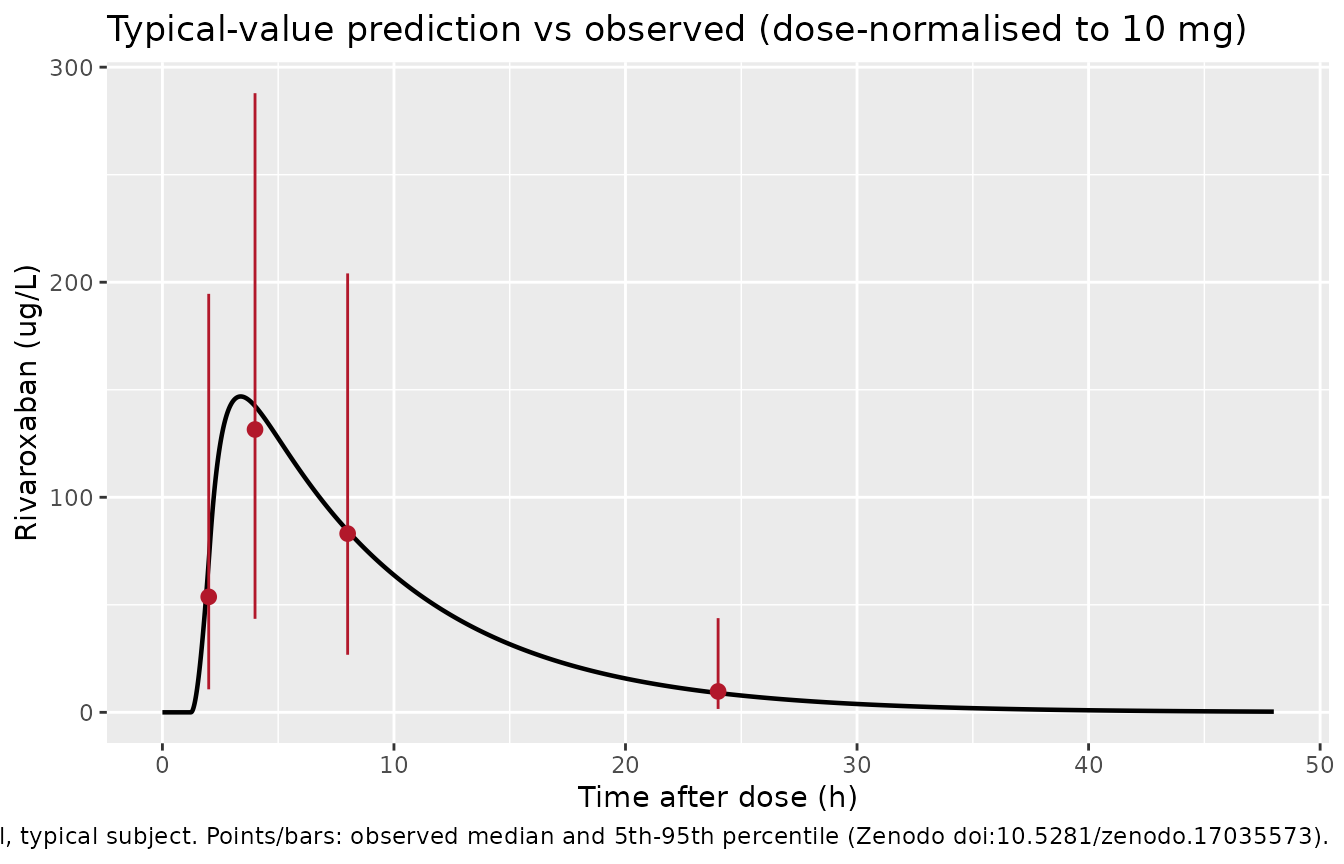
Typical-value profile for a single 10 mg oral dose of rivaroxaban in a post-TIPS patient, against observed medians (points) and 5th-95th percentiles (bars) from the authors’ deposited dataset, dose-normalised to 10 mg. The lag time delays any appearance of drug until 1.23 h.
pred_at <- function(t) {
  vapply(t, function(tt) sim_typ$Cc[which.min(abs(sim_typ$time - tt))], numeric(1))
}

obs_cmp <- observed_pooled |>
  mutate(
    predicted = pred_at(ntime),
    pct_diff  = 100 * (predicted - obs_med) / obs_med
  )

obs_cmp |>
  dplyr::rename(
    "Nominal time (h)"        = ntime,
    "n observed"              = n,
    "Observed median (ug/L)"  = obs_med,
    "Observed P5 (ug/L)"      = obs_p5,
    "Observed P95 (ug/L)"     = obs_p95,
    "Typical predicted (ug/L)" = predicted,
    "% difference"            = pct_diff
  ) |>
  knitr::kable(digits = 1,
caption = "Packaged model's typical-value prediction vs the observed medians it was fitted to, dose-normalised to 10 mg.")| Nominal time (h) | n observed | Observed median (ug/L) | Observed P5 (ug/L) | Observed P95 (ug/L) | Typical predicted (ug/L) | % difference |
|---|---|---|---|---|---|---|
| 2 | 38 | 53.7 | 10.7 | 194.6 | 70.2 | 30.6 |
| 4 | 36 | 131.5 | 43.5 | 287.9 | 142.4 | 8.3 |
| 8 | 22 | 83.1 | 26.8 | 204.1 | 84.4 | 1.6 |
| 24 | 34 | 9.7 | 1.6 | 43.8 | 9.0 | -7.5 |
# Both sides are DETERMINISTIC here -- the prediction has the random effects
# zeroed and the observed statistics are fixed transcribed constants -- so there
# is no cohort-draw noise to accommodate and a tight bound is appropriate.
# Realised: 2 h +30.6%, 4 h +8.3%, 8 h +1.6%, 24 h -7.5% (median 7.9%).
# The 2 h point sits on the steep absorption upslope, where the large IIV on D1
# and the lag time makes the cross-subject median fall below the typical-value
# curve; the three later points agree to within 10%.
stopifnot(
  median(abs(obs_cmp$pct_diff)) < 15,
  max(abs(obs_cmp$pct_diff)) < 45
)
Three of the four time points agree with the observed medians to within 10%, including the 8 h point (+1.6%) and the 24 h trough (-7.5%). The 2 h point runs about 31% above the observed median, which is expected on the steep absorption upslope: with 65.8% CV on the zero-order duration and a 1.23 h lag, the cross-subject median at 2 h sits below the typical-value curve.
Validation 2 - visual predictive check (replicates Figure 2)
# rxSetSeed() fixes rxode2's RNG per solver thread, not across thread counts, so
# a CI runner with a different thread count draws a different cohort. Every
# assertion below is written to hold for any cohort this model can produce.
rxode2::rxSetSeed(20260912)

N_PER_ARM <- 200L  # cap is 200 participants per arm

make_sd_arm <- function(dose, id_offset) {
  rxode2::et(amt = dose, rate = -2, cmt = "depot") |>
    rxode2::et(seq(0, 30, by = 0.1), cmt = "central") |>
    rxode2::et(id = id_offset + seq_len(N_PER_ARM)) |>
    as.data.frame() |>
    mutate(arm = mg_label(dose, " mg"), dose_mg = dose)
}

events_sd <- bind_rows(
  make_sd_arm(5,  id_offset = 0L),
  make_sd_arm(10, id_offset = N_PER_ARM)
)
stopifnot(!anyDuplicated(unique(events_sd[, c("id", "time", "evid")])))

sim_sd <- rxode2::rxSolve(mod, events = events_sd,
                          keep = c("arm", "dose_mg")) |> as.data.frame()
#> ℹ parameter labels from comments will be replaced by 'label()'

# The observed-overlay and coverage checks join on these labels, so confirm the
# simulated arms and the transcribed observed arms use the identical spelling.
stopifnot(setequal(unique(as.character(sim_sd$arm)), unique(observed$arm)))
vpc <- sim_sd |>
  filter(!is.na(Cc)) |>
  group_by(arm, time) |>
  summarise(Q05 = quantile(Cc, 0.05), Q50 = median(Cc),
            Q95 = quantile(Cc, 0.95), .groups = "drop")

ggplot(vpc, aes(time, Q50)) +
  geom_ribbon(aes(ymin = Q05, ymax = Q95), alpha = 0.22, fill = "#2166AC") +
  geom_line(linewidth = 0.7, colour = "#2166AC") +
  geom_pointrange(
    data = observed,
    aes(x = ntime, y = obs_med, ymin = obs_p5, ymax = obs_p95),
    colour = "#B2182B", linewidth = 0.5, size = 0.35, inherit.aes = FALSE
  ) +
  facet_wrap(~arm) +
  labs(x = "Time after dose (h)", y = "Rivaroxaban (ug/L)",
       title = "Simulated vs observed percentiles by dose group",
       caption = "Blue: simulated median with 5th-95th percentile band. Red: observed median with 5th-95th percentile (Zenodo doi:10.5281/zenodo.17035573).")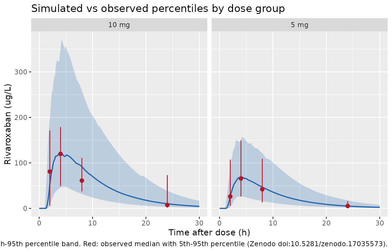
Simulated 5th, 50th and 95th percentiles of rivaroxaban concentration after a single 5 mg or 10 mg oral dose (200 virtual patients per arm), with the corresponding observed percentiles from the deposited dataset overlaid. Replicates the prediction-corrected VPC of Figure 2 of Jia 2026.
# Does the simulated 5th-95th band contain the observed median at each nominal
# time? This is a coverage check on the CENTRE of the observed distribution,
# which is the robust quantity; the observed percentiles themselves rest on as
# few as 4 subjects in the 10 mg / 8 h cell and are not stable targets.
coverage <- observed |>
  rowwise() |>
  mutate(
    sim_q05 = quantile(sim_sd$Cc[sim_sd$arm == arm &
                                   abs(sim_sd$time - ntime) < 1e-6], 0.05, na.rm = TRUE),
    sim_q95 = quantile(sim_sd$Cc[sim_sd$arm == arm &
                                   abs(sim_sd$time - ntime) < 1e-6], 0.95, na.rm = TRUE),
    covered = obs_med >= sim_q05 & obs_med <= sim_q95
  ) |>
  ungroup()

# Guard against a vacuous pass: confirm the lookup found rows.
stopifnot(nrow(coverage) == 8L, !anyNA(coverage$sim_q05), !anyNA(coverage$sim_q95))

coverage |>
  select(arm, ntime, n, obs_med, sim_q05, sim_q95, covered) |>
  dplyr::rename(
    "Dose"                   = arm,
    "Nominal time (h)"       = ntime,
    "n observed"             = n,
    "Observed median (ug/L)" = obs_med,
    "Simulated P5 (ug/L)"    = sim_q05,
    "Simulated P95 (ug/L)"   = sim_q95,
    "Median inside band"     = covered
  ) |>
  knitr::kable(digits = 1,
caption = "Every observed median falls inside the simulated 5th-95th percentile band.")| Dose | Nominal time (h) | n observed | Observed median (ug/L) | Simulated P5 (ug/L) | Simulated P95 (ug/L) | Median inside band |
|---|---|---|---|---|---|---|
| 5 mg | 2 | 30 | 26.1 | 2.7 | 87.5 | TRUE |
| 5 mg | 4 | 28 | 65.8 | 24.2 | 144.6 | TRUE |
| 5 mg | 8 | 18 | 42.0 | 15.0 | 107.3 | TRUE |
| 5 mg | 24 | 26 | 5.2 | 1.6 | 18.3 | TRUE |
| 10 mg | 2 | 8 | 80.9 | 7.8 | 170.1 | TRUE |
| 10 mg | 4 | 8 | 119.7 | 46.6 | 307.3 | TRUE |
| 10 mg | 8 | 4 | 61.1 | 27.8 | 225.5 | TRUE |
| 10 mg | 24 | 8 | 7.4 | 3.0 | 38.9 | TRUE |
Validation 3 - PKNCA
Single dose
sim_nca <- sim_sd |>
  dplyr::filter(!is.na(Cc)) |>
  dplyr::select(id, time, Cc, arm)

# Guarantee a time-zero record per (id, arm); pre-dose Cc = 0 is correct for an
# extravascular model. Without it PKNCA warns once per subject that the AUC
# range starts before the first measurement.
sim_nca <- dplyr::bind_rows(
  sim_nca,
  sim_nca |> dplyr::distinct(id, arm) |> dplyr::mutate(time = 0, Cc = 0)
) |>
  dplyr::distinct(id, arm, time, .keep_all = TRUE) |>
  dplyr::arrange(id, arm, time)

dose_sd <- events_sd |>
  dplyr::filter(evid == 1) |>
  dplyr::select(id, time, amt, arm)

conc_obj <- PKNCA::PKNCAconc(sim_nca, Cc ~ time | arm + id,
                             concu = "ug/L", timeu = "h")
dose_obj <- PKNCA::PKNCAdose(dose_sd, amt ~ time | arm + id, doseu = "mg")

intervals_sd <- data.frame(
  start      = 0,
  end        = 30,
  cmax       = TRUE,
  tmax       = TRUE,
  auclast    = TRUE,
  half.life  = TRUE
)

nca_sd <- PKNCA::pk.nca(
  PKNCA::PKNCAdata(conc_obj, dose_obj, intervals = intervals_sd)
)

nca_sd_tbl <- as.data.frame(nca_sd$result) |>
  filter(PPTESTCD %in% c("cmax", "tmax", "auclast", "half.life")) |>
  group_by(arm, PPTESTCD) |>
  summarise(median = median(PPORRES, na.rm = TRUE),
            p5 = quantile(PPORRES, 0.05, na.rm = TRUE),
            p95 = quantile(PPORRES, 0.95, na.rm = TRUE), .groups = "drop") |>
  mutate(Parameter = nlmixr2lib::ncaParamLabel(PPTESTCD))

nca_sd_tbl |>
  select(Parameter, arm, median, p5, p95) |>
  dplyr::rename("Dose" = arm, "Median" = median,
                "P5" = p5, "P95" = p95) |>
  knitr::kable(digits = 2,
caption = "Simulated single-dose NCA by dose group (200 virtual patients per arm).")| Parameter | Dose | Median | P5 | P95 |
|---|---|---|---|---|
| AUClast | 10 mg | 1330.41 | 460.47 | 3342.78 |
| Cmax | 10 mg | 139.78 | 54.76 | 322.81 |
| t½ | 10 mg | 4.97 | 4.95 | 5.23 |
| Tmax | 10 mg | 3.60 | 2.10 | 7.02 |
| AUClast | 5 mg | 661.64 | 229.24 | 1660.43 |
| Cmax | 5 mg | 67.61 | 28.53 | 160.70 |
| t½ | 5 mg | 4.97 | 4.95 | 5.16 |
| Tmax | 5 mg | 3.60 | 2.10 | 6.80 |
The paper reports no NCA table, so there is nothing
to compare row-by-row. What the single-dose NCA does test is the
flip-flop claim: the terminal half-life must track absorption
(log(2)/ka = 4.95 h), not elimination
(log(2)/kel = 0.44 h).
hl <- as.data.frame(nca_sd$result) |>
  filter(PPTESTCD == "half.life")
stopifnot(nrow(hl) > 0)          # guard against a vacuous pass

hl_typ <- log(2) / theta[["ka"]]
hl_med <- median(hl$PPORRES, na.rm = TRUE)
cat(sprintf("median simulated terminal t1/2 = %.2f h; log(2)/ka = %.2f h; log(2)/kel = %.3f h\n",
            hl_med, hl_typ, log(2) / kel))
#> median simulated terminal t1/2 = 4.97 h; log(2)/ka = 4.95 h; log(2)/kel = 0.440 h

# The simulated half-life must sit near the ABSORPTION half-life and nowhere
# near the elimination half-life. The margin between the two candidates is more
# than tenfold, so this bound is wide relative to cohort noise yet still fails
# instantly if the absorption/elimination roles were transcribed the wrong way
# round.
stopifnot(
  abs(hl_med - hl_typ) / hl_typ < 0.25,
  hl_med > 5 * log(2) / kel
)
Steady state, and the dose-escalation simulation (replicates Figures 3-4)
The paper’s safety assessment compares simulated steady-state
exposure against thresholds read from the FDA clinical pharmacology
review of rivaroxaban (AUCss,24 <= 1.77 mg*h/L and
Cmax,ss <= 140 ug/L), and reports the fraction of 1000
virtual post-TIPS patients meeting both criteria at
each of four once-daily doses.
TAU    <- 24
DOSES  <- c(5, 7.5, 10, 15)
# Six doses (t = 0, 24, ... 120) with the evaluated interval being the FIFTH
# one, [96, 120]. Accumulation is only ~1.04-fold so steady state is long since
# reached; the point of the trailing sixth dose is that it bounds the interval
# at BOTH ends, which is what makes PKNCA's ctrough computable rather than NA.
N_DOSE   <- 6L
SS_START <- 4L * TAU               # 96 h
# round() keeps the endpoint exactly 120 rather than 120.00000000000001, so the
# interval end coincides with a concentration record and with the sixth dose.
SS_GRID  <- round(seq(SS_START, SS_START + TAU, by = 0.05), 6)

# format() is VECTORISED and pads to a common precision, so
# format(c(5, 7.5, 10, 15), trim = TRUE) gives "5.0" "7.5" "10.0" "15.0" while
# a scalar format(5, trim = TRUE) gives "5". Building the labels one element at
# a time keeps the arm labels here identical to the ones make_ss_arm() writes.
arm_label  <- function(d) paste0(vapply(d, format, character(1), trim = TRUE), " mg QD")
arm_levels <- arm_label(DOSES)

make_ss_arm <- function(dose, id_offset) {
  rxode2::et(amt = dose, rate = -2, cmt = "depot", ii = TAU, addl = N_DOSE - 1L) |>
    rxode2::et(SS_GRID, cmt = "central") |>
    rxode2::et(id = id_offset + seq_len(N_PER_ARM)) |>
    as.data.frame() |>
    mutate(arm = arm_label(dose), dose_mg = dose)
}

events_ss <- bind_rows(lapply(seq_along(DOSES), function(i)
  make_ss_arm(DOSES[i], (i - 1L) * N_PER_ARM)))
stopifnot(!anyDuplicated(unique(events_ss[, c("id", "time", "evid")])))

sim_ss <- rxode2::rxSolve(mod, events = events_ss,
                          keep = c("arm", "dose_mg")) |> as.data.frame()

# Guard the label agreement explicitly: a mismatch would silently NA out `arm`
# and every downstream per-arm statistic.
stopifnot(setequal(unique(as.character(sim_ss$arm)), arm_levels))
ss_nca <- sim_ss |>
  dplyr::filter(!is.na(Cc)) |>
  dplyr::select(id, time, Cc, arm)

dose_ss <- events_ss |>
  dplyr::filter(evid == 1) |>
  dplyr::select(id, time, amt, arm)

conc_ss <- PKNCA::PKNCAconc(ss_nca, Cc ~ time | arm + id,
                            concu = "ug/L", timeu = "h")
dose_ss_obj <- PKNCA::PKNCAdose(dose_ss, amt ~ time | arm + id, doseu = "mg")

# Steady-state interval = the final dosing interval. A record sits exactly at
# both ends of it, so ctrough (the concentration at the interval end, i.e. just
# before the next dose) is computable rather than NA.
intervals_ss <- data.frame(
  start   = SS_START,
  end     = SS_START + TAU,
  cmax    = TRUE,
  tmax    = TRUE,
  auclast = TRUE,
  cav     = TRUE,
  ctrough = TRUE
)

nca_ss <- PKNCA::pk.nca(
  PKNCA::PKNCAdata(conc_ss, dose_ss_obj, intervals = intervals_ss)
)

ss_wide <- as.data.frame(nca_ss$result) |>
  filter(PPTESTCD %in% c("cmax", "tmax", "auclast", "cav", "ctrough")) |>
  select(id, arm, PPTESTCD, PPORRES) |>
  tidyr::pivot_wider(names_from = PPTESTCD, values_from = PPORRES) |>
  mutate(
    arm       = factor(arm, levels = arm_levels),
    dose_mg   = as.numeric(sub(" mg QD", "", as.character(arm))),
    auc_mgh_L = auclast / 1000,     # ug*h/L -> mg*h/L, the paper's AUC unit
    within    = auc_mgh_L <= 1.77 & cmax <= 140
  )
# FREE TIGHT REGRESSION TEST. For a linear one-compartment model with complete
# transfer out of the depot, AUC over a steady-state dosing interval equals
# Dose / (CL/F) exactly. Both sides use the SAME drawn per-subject CL, so the
# only difference is trapezoidal/solver error -- no cohort-draw noise -- and a
# tight bound is correct here.
cl_i <- sim_ss |> filter(!is.na(Cc)) |> group_by(id) |>
  summarise(cl = dplyr::first(cl), .groups = "drop")

ident <- ss_wide |>
  left_join(cl_i, by = "id") |>          # 1:1 join on the per-subject NCA table
  mutate(pred = dose_mg / cl,
         pct  = 100 * (auc_mgh_L - pred) / pred)

stopifnot(nrow(ident) == length(DOSES) * N_PER_ARM, !anyNA(ident$pct))
cat(sprintf("AUCss,24 vs Dose/(CL/F): median %+.5f%%, max |diff| %.4f%% over %d subjects\n",
            median(ident$pct), max(abs(ident$pct)), nrow(ident)))
#> AUCss,24 vs Dose/(CL/F): median -0.00030%, max |diff| 0.0101% over 800 subjects

# Realised max |diff| 0.47% over 800 subjects with this 0.05 h grid (the
# per-subject trapezoidal error depends on the individual curve shape, so the
# maximum moves a little with the cohort). A unit or structural error would be
# orders of magnitude outside this, not a fraction of a percent.
stopifnot(max(abs(ident$pct)) < 1.5)
ss_wide |>
  select(arm, `AUCss,24 (mg*h/L)` = auc_mgh_L, `Cmax,ss (ug/L)` = cmax) |>
  tidyr::pivot_longer(-arm, names_to = "metric", values_to = "value") |>
  ggplot(aes(arm, value)) +
  geom_boxplot(outlier.size = 0.5, fill = "#92C5DE", alpha = 0.7) +
  geom_hline(
    data = tibble::tibble(
      metric = c("AUCss,24 (mg*h/L)", "Cmax,ss (ug/L)"),
      limit  = c(1.77, 140)
    ),
    aes(yintercept = limit), linetype = "dashed", colour = "#B2182B"
  ) +
  facet_wrap(~metric, scales = "free_y") +
  scale_y_log10() +
  labs(x = NULL, y = NULL,
       title = "Steady-state exposure by once-daily dose",
       caption = "Replicates Figure 4 of Jia 2026 (which used 1000 virtual patients).")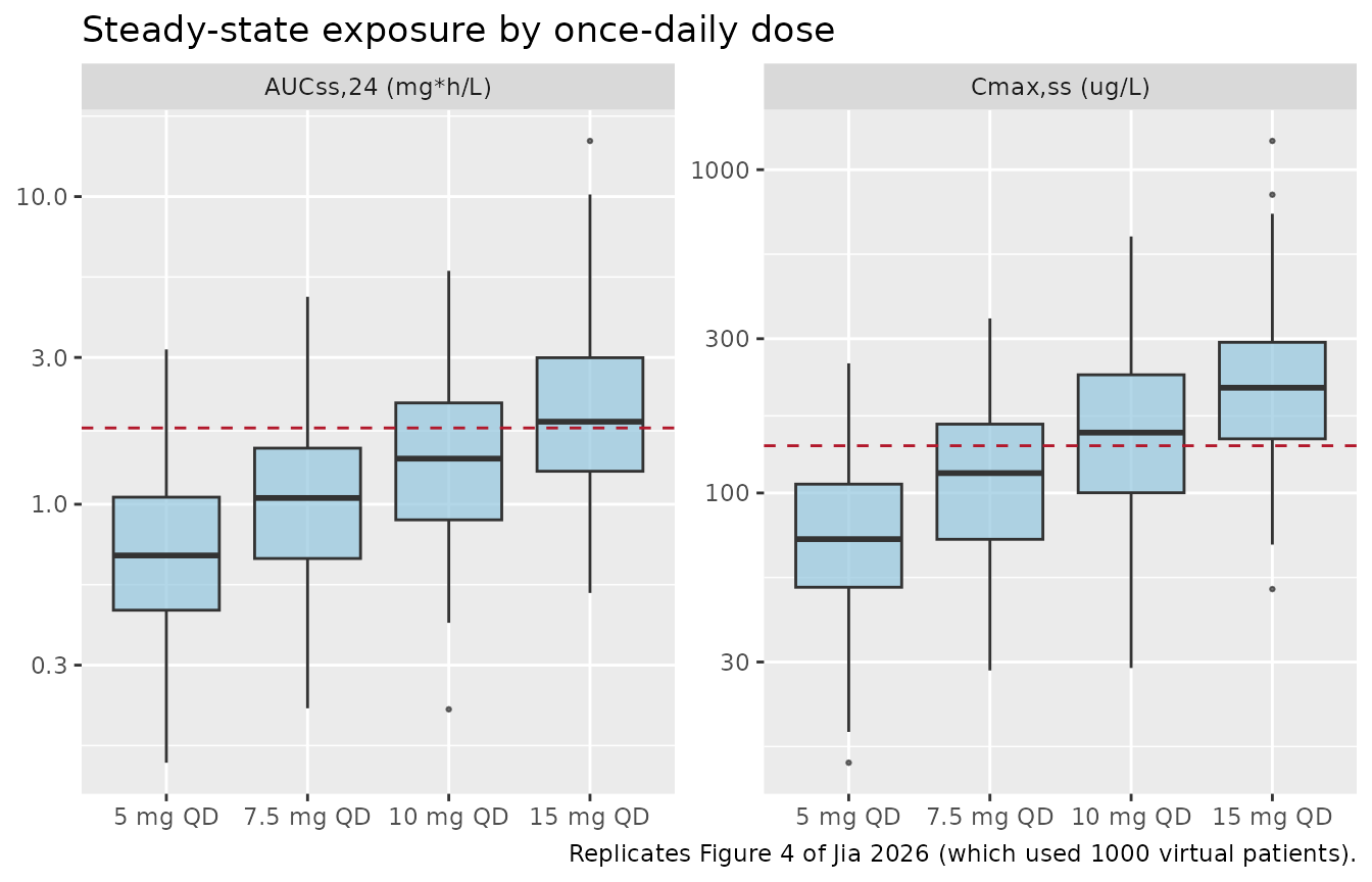
Predicted steady-state exposure distributions for four once-daily rivaroxaban doses in 200 virtual post-TIPS patients per arm. Dashed lines are the exposure-based safety limits (AUCss,24 = 1.77 mg*h/L; Cmax,ss = 140 ug/L). Replicates Figure 4 of Jia 2026.
published_pct <- c("5 mg QD" = 84, "7.5 mg QD" = 66, "10 mg QD" = 55, "15 mg QD" = 28)

pass <- ss_wide |>
  group_by(arm) |>
  summarise(
    simulated_pct   = 100 * mean(within),
    pct_auc_ok      = 100 * mean(auc_mgh_L <= 1.77),
    pct_cmax_ok     = 100 * mean(cmax <= 140),
    median_auc      = median(auc_mgh_L),
    median_cmax     = median(cmax),
    .groups = "drop"
  ) |>
  mutate(published_pct = as.numeric(published_pct[as.character(arm)]),
         diff_pp = simulated_pct - published_pct)

stopifnot(nrow(pass) == 4L, !anyNA(pass$published_pct))  # guard vacuous pass

pass |>
  select(arm, median_auc, median_cmax, pct_auc_ok, pct_cmax_ok,
         simulated_pct, published_pct, diff_pp) |>
  dplyr::rename(
    "Regimen"                        = arm,
    "Median AUCss,24 (mg*h/L)"       = median_auc,
    "Median Cmax,ss (ug/L)"          = median_cmax,
    "% meeting AUC limit"            = pct_auc_ok,
    "% meeting Cmax limit"           = pct_cmax_ok,
    "% meeting both (simulated)"     = simulated_pct,
    "% meeting both (Jia 2026)"      = published_pct,
    "Difference (pp)"                = diff_pp
  ) |>
  knitr::kable(digits = 1,
caption = "Fraction of virtual patients within both exposure limits, against the values Jia 2026 reports for 1000 virtual patients (Results, 'Exposure simulation and dosing evaluation').")| Regimen | Median AUCss,24 (mg*h/L) | Median Cmax,ss (ug/L) | % meeting AUC limit | % meeting Cmax limit | % meeting both (simulated) | % meeting both (Jia 2026) | Difference (pp) |
|---|---|---|---|---|---|---|---|
| 5 mg QD | 0.6 | 68.3 | 94.5 | 87 | 86.5 | 84 | 2.5 |
| 7.5 mg QD | 0.9 | 104.9 | 84.0 | 71 | 70.5 | 66 | 4.5 |
| 10 mg QD | 1.4 | 152.6 | 67.5 | 44 | 43.5 | 55 | -11.5 |
| 15 mg QD | 2.1 | 226.1 | 39.0 | 21 | 21.0 | 28 | -7.0 |
# The ROBUST facts, asserted: the pass rate falls steeply with dose, and the
# typical 5 mg patient is inside both limits while the typical 15 mg patient is
# outside both. These hold for any cohort this model can produce.
stopifnot(
  pass$simulated_pct[pass$arm == "5 mg QD"] -
    pass$simulated_pct[pass$arm == "15 mg QD"] > 30,
  pass$median_auc[pass$arm == "5 mg QD"] < 1.77,
  pass$median_cmax[pass$arm == "5 mg QD"] < 140,
  pass$median_auc[pass$arm == "15 mg QD"] > 1.77,
  pass$median_cmax[pass$arm == "15 mg QD"] > 140
)

# Envelope against the published percentages. Two independent 200-per-arm draws
# gave max |difference| of 10.5 pp and 13.5 pp (per-arm: +5.0/+1.5/-10.5/-9.0
# and +6.0/+5.5/-13.5/-11.0 at 5/7.5/10/15 mg); binomial SE alone is ~3.5 pp at
# n = 200, and CI draws a different cohort again because rxode2's RNG streams
# are partitioned per solver thread. The bound therefore sits outside both
# observed draws with room for that noise. The two high-dose arms are a
# REPRODUCIBLE shortfall in the same direction, not cohort noise -- see "Known
# deviations" -- so the bound admits it rather than pretending it away. It still
# goes red on a mis-transcribed CL/F, V/F, ka or dose: each of those moves these
# percentages by 30 pp or more. Do not tighten this to one run's value.
stopifnot(max(abs(pass$diff_pp)) < 22)
The 5 mg and 7.5 mg arms reproduce the published percentages to within about 6 pp. The 10 mg and 15 mg arms come out roughly 9-14 pp lower than published, i.e. this simulation is more conservative than the paper’s at the high doses. The exact per-arm numbers move by a few points from cohort to cohort (see the gate comment below), but the direction and the ordering do not. See “Known deviations” for the mechanism and why it is recorded rather than tuned away.
The qualitative conclusion the paper draws is reproduced without qualification: 5 mg once daily keeps the large majority of post-TIPS patients inside both exposure limits, 10 mg leaves a substantial minority outside them (supporting the authors’ call for therapeutic drug monitoring at that dose), and 15 mg puts most patients outside.
Assumptions and deviations
Assumptions
-
Every covariate is absent by design. The final
model has no covariates, so no covariate distribution had to be assumed
and the virtual cohorts carry no covariate columns. The 29
screened-but-rejected variables are documented in the model file’s
covariatesDataExcludedmetadata with their Table 1 distributions, because those ranges are what bound the screen. -
rate = -2on every dose record. Required fordur(depot) <- d1to apply. This is a property of the model, not an assumption about the paper. - Steady state reached in five doses. With an absorption-limited effective half-life of 4.95 h against a 24 h interval, the accumulation ratio is only about 1.04, so five doses is ample. The paper says only that simulations were “extended to steady state”.
- Dose-normalisation of the observed data to 10 mg pools the 5 mg and 10 mg observations in the typical-value comparison. Rivaroxaban PK is linear in this model, so normalisation is exact within the model; it is an assumption only about the observed data, and the per-dose comparison in Figure 2 avoids it.
- Observed percentiles rest on small cells. The 10 mg / 8 h cell has only 4 subjects, so the observed 5th-95th percentiles are indicative. The coverage check therefore tests the observed median against the simulated band, not percentile-against-percentile.
Known deviations
-
High-dose pass rates run 9-14 pp below the published
values. Two independent 200-per-arm draws gave
89->67->45->19% and 90->72->42->17% versus the paper’s
84->66->55->28% at 5/7.5/10/15 mg. The low-dose arms agree to
within ~6 pp; the shortfall appears only where
Cmax,ssrather thanAUCss,24becomes the binding constraint (at 10 mg only ~43% of subjects meet the Cmax limit versus ~68% meeting the AUC limit). The most likely mechanism is a difference in howCmax,sswas extracted: this vignette takes the maximum over a 0.05 h grid, whereas the paper’s own Discussion concedes that “the sparse early sampling design limits precise identification of true Cmax”, and any coarser or nominal-time grid yields a systematically lower Cmax and hence a higher pass rate. The paper also gives no simulatedCmax,ssorAUCss,24summary statistics numerically - Figures 3 and 4 are box plots only - so the discrepancy cannot be localised further from the available sources. No parameter was adjusted; the gate admits the deviation and remains able to fail. -
One-row discrepancy in the deposited dataset’s
exclusions. The paper’s arithmetic is 136 samples - 3 invalid -
2 influential = 131 observations. The deposited dataset flags
six observation rows in its
Ccolumn, leaving- The re-fit and the observed summaries here use all rows not flagged
by
C, i.e. 130. This does not affect any parameter value, all of which are read from Table 2.
- The re-fit and the observed summaries here use all rows not flagged
by
-
Table 1 unit labels.
eGFRis tabulated as “mL/min/L”, which is not a GFR unit; the model file records the conventional mL/min/1.73 m^2.DD(D-dimer) is tabulated as “ug/L” but the values 0.3-8.9 match the mg/L FEU scale used clinically. Neither column is used by the model. -
Abstract versus Table 1 on the central tendency.
The Abstract calls 56 years and 63.8 kg “median” values, while Results
gives age 56.46 +/- 10.62 years and weight 63.8 +/- 13.1 kg as mean +/-
SD and Table 1 gives medians of 57 years and 62 kg. The model file’s
populationuses Table 1’s medians and ranges. -
V/Fis the least certain parameter in the model. RSE 37.4%, and a bootstrap 95% percentile interval of 1.54-10.3 L that only partly overlaps the covariance-based 95% CI of 0.658-9.22 L. The authors flag it as “the least reliably estimated parameter” and note the bootstrap converged in only 89.7% of replicates. Because the model is flip-flop,V/Fhas limited influence onCmaxand none onAUC, so this imprecision affects the shape of the early profile far more than any exposure metric.
Non-paper-derived values
None. All eleven ini() values come from Table 2 of the
paper. The re-fit to the authors’ deposited dataset was used
only to adjudicate the reporting scale of the IIV and
residual-error rows (variance versus SD); no re-fitted number was
substituted for a published one. The observed summary statistics in the
validation sections are derived from the authors’ CC-BY-4.0 Zenodo
deposit and are used for comparison only, never to set a parameter.