Model and source
- Citation: Li J, Hu P, Zhou L, Nagahama F, Chen R. Population pharmacokinetic analysis of transdermal granisetron in healthy Chinese and Caucasian volunteers. Front Pharmacol. 2023;14:1154026. doi:10.3389/fphar.2023.1154026
- Description: One-compartment population PK model for the granisetron transdermal delivery system (GTDS, Sancuso 34.3 mg/52 cm2 patch) in healthy Caucasian volunteers, with first-order absorption from the patch (no lag time) and first-order elimination; no covariates retained (Li 2023)
- Article: https://doi.org/10.3389/fphar.2023.1154026 (open access, CC BY)
The granisetron transdermal delivery system (GTDS, marketed as Sancuso) is a 34.3 mg/52 cm^2 patch applied to the upper arm 24-48 h before chemotherapy for prophylaxis of chemotherapy-induced nausea and vomiting (CINV). Li 2023 pooled four Caucasian healthy-volunteer studies to build a population PK model, then used that model to simulate a large Caucasian control group under the design of a separate Chinese healthy-volunteer study, in order to test whether a dose adjustment is needed in the Chinese population. The conclusion was that no dose adjustment is required.
Population
The model was fit to 1372 plasma granisetron concentrations from 112 healthy Caucasian volunteers enrolled in four sponsor studies (Li 2023 Table 1: 392MD/11/C n = 12, 392MD/26/C n = 24, 392MD/40/C n = 59, 392MD/43/C n = 16). Every subject received a single 34.3 mg/52 cm^2 patch, worn for 6-9 days depending on the study, with study-specific sampling schedules running from pre-dose out to 120-216 h post-application. Pooled Caucasian baseline characteristics were age 43.01 +/- 17.80 years, weight 70.54 +/- 16.13 kg, height 169.51 +/- 9.69 cm, BMI 24.39 +/- 4.43 kg/m^2, and 42.86% female (Li 2023 Section 3.1).
A fifth study (SP-0102) contributed 24 healthy Chinese male volunteers (age 27.13 +/- 4.07 years, weight 65.07 +/- 5.67 kg, sampling to 240 h; Li 2023 Table 2). Those data were not used for parameter estimation – they served as the external comparison cohort against which the Caucasian model’s predictions were judged (Li 2023 Sections 2.3.2 and 3.4).
Parameters were estimated in Phoenix NLME 1.30 with FOCE ELS.
The same information is available programmatically via
readModelDb("Li_2023_granisetron")()$population.
Source trace
Per-parameter origin is recorded as an in-file comment next to each
ini() entry in
inst/modeldb/specificDrugs/Li_2023_granisetron.R. The table
below collects them for review.
| Equation / parameter | Value | Source location |
|---|---|---|
| Structural model | 1-cmt, first-order absorption (no lag), first-order elimination | Li 2023 Section 3.2 and Figure 1; selected over 2-cmt on AIC/BIC (1-cmt AIC 4895.1498 / BIC 4931.6616 vs 2-cmt AIC 4963.0765 / BIC 5020.4522) |
d/dt(depot) |
-ka * depot |
Li 2023 Eq 4: dAa/dt = -ka x Aa |
d/dt(central) |
ka * depot - kel * central |
Li 2023 Eq 5: dA1/dt = -CL x C + ka x Aa |
Cc |
central / vc |
Li 2023 Eq 6: C = A1/V |
| Error model | additive | Li 2023 Eq 7 (Cobs = C + epsilon) and Section 3.2 (additive selected over proportional and mixed) |
| IIV form | exponential (log-normal) | Li 2023 Eqs 8-10: ka = tvka x exp(eta_ka), V = tvV x exp(eta_V), CL = tvCL x exp(eta_CL) |
lka (Ka) |
log(0.0179879) 1/h |
Table 3 fixed effect: Ka = 0.0179879 (RSE 3.63%); bootstrap mean 0.017966084, 95% CI 0.016469625-0.019216464 |
lcl (CL/F) |
log(31.3163) L/h |
Table 3 fixed effect: CL = 31316.3 mL/h (RSE 5.52%); bootstrap mean 31042.673, 95% CI 26407.14-36914.471 mL/h; Abstract restates 31316.3 mL/h |
lvc (V/F) |
log(6299.03) L |
Table 3 fixed effect: V = 6299030 mL (RSE 13.12%); bootstrap mean 6351196.5, 95% CI 4962557.7-8105176.7 mL; Abstract restates 6299.03 L |
etalka |
4.74078e-11 |
Table 3 random effect Ka (RSE 149.11%); bootstrap 95% CI 0.00000-0.00000 |
etalcl |
0.25423392 |
Table 3 random effect CL (RSE 20.19%); bootstrap 95% CI 0.1536138-0.3548540 (= 53.8% CV) |
etalvc |
1.5462161 |
Table 3 random effect V (RSE 12.11%); bootstrap 95% CI 1.179257-1.9131749 (= 192% CV) |
addSd |
1.18094 ng/mL |
Table 3 residual error sigma (RSE 10.17%); bootstrap mean 1.1706386, 95% CI 0.94536484-1.4335495 |
| Covariate screen (none retained) | AGE, WT, HT, BMI, SEXF | Li 2023 Sections 2.2 and 3.2: forward inclusion dOFV > 3.84 then backward elimination dOFV > 6.64; none significant |
| Reference NCA values | Table 4 | Li 2023 Table 4 (Chinese observed median; Caucasian simulated median with P5:P95) |
| Concentration units | ng/mL | Li 2023 Figures 2-4 axis labels (DV/IPRED/PRED in ng/mL) |
Units
Li 2023 Table 3 reports V in mL and CL in
mL/h while the concentration axes of Figures 2-4 are in ng/mL. Because 1
ug/L is identically 1 ng/mL, the packaged model expresses
vc in L and cl in L/h and doses in
ug, so Cc <- central / vc lands
directly on the paper’s ng/mL scale with no scale factor. A 34.3 mg
patch is therefore dosed as amt = 34300.
mod <- readModelDb("Li_2023_granisetron")
rxode2::rxode2(mod)$units
#> ℹ parameter labels from comments will be replaced by 'label()'
#> $time
#> [1] "h"
#>
#> $dosing
#> [1] "ug"
#>
#> $concentration
#> [1] "ng/mL"
Virtual cohort
Original observed data are not publicly available. Two virtual cohorts are simulated, each of 200 subjects (the per-arm cap for validation vignettes). The model carries no covariates, so the cohorts differ only in sampling design.
-
SP-0102design – the sampling schedule of the Chinese study that Li 2023 used as the comparison design (pre-dose and 6, 12, 24, 48, 72, 96, 120, 144, 150, 168, 192, 216, 240 h; Li 2023 Table 1). Used for the NCA comparison against Table 4 and for the Figure 6 replication. -
densedesign – a fine 0-240 h grid used only to draw smooth prediction-interval ribbons for the Figure 5 (VPC) replication.
set.seed(20230626)

n_per_arm <- 200L

# SP-0102 sampling times (Li 2023 Table 1, study SP-0102)
times_sp0102 <- c(0, 6, 12, 24, 48, 72, 96, 120, 144, 150, 168, 192, 216, 240)
times_dense <- seq(0, 240, by = 4)

patch_dose_ug <- 34300 # 34.3 mg/52 cm^2 patch content, expressed in ug

make_cohort <- function(n, obs_times, design, id_offset = 0L) {
  subj <- tibble(id = id_offset + seq_len(n), design = design)

  doses <- subj |>
    mutate(
      time = 0,
      amt = patch_dose_ug,
      evid = 1L,
      cmt = "depot"
    )

  # Observation rows point at the ODE state `central`, never at the algebraic
  # observable `Cc`; rxode2 returns Cc as an output column regardless.
  obs <- subj |>
    tidyr::crossing(time = obs_times) |>
    mutate(
      amt = NA_real_,
      evid = 0L,
      cmt = "central"
    )

  bind_rows(doses, obs) |>
    arrange(id, time, desc(evid))
}

events <- bind_rows(
  make_cohort(n_per_arm, times_sp0102, "SP-0102", id_offset = 0L),
  make_cohort(n_per_arm, times_dense, "dense", id_offset = 1000L)
)

stopifnot(!anyDuplicated(unique(events[, c("id", "time", "evid")])))
Simulation
simdf <- rxode2::rxSolve(mod, events = events, keep = "design") |>
  as.data.frame()
#> ℹ parameter labels from comments will be replaced by 'label()'

# rxode2 returns `Cc` as the individual prediction (IPRED) and `sim` as the
# simulated observation, i.e. Cc plus the additive residual error of Eq 7. A real
# assay cannot report a negative concentration, so the observation scale is
# truncated at zero.
stopifnot(all(c("Cc", "sim") %in% names(simdf)))
simdf <- simdf |>
  mutate(Cc_dv = pmax(sim, 0))

sim_sp <- filter(simdf, design == "SP-0102")
sim_dense <- filter(simdf, design == "dense")
The typical-value (all etas zero) profile fixes the model’s central tendency:
ev_typ <- rxode2::et(amt = patch_dose_ug, cmt = "depot") |>
  rxode2::et(seq(0, 240, by = 1), cmt = "central")

sim_typ <- rxode2::rxSolve(mod, ev_typ, omega = NA, sigma = NA) |>
  as.data.frame()

tibble(
  `Typical Cmax (ng/mL)` = max(sim_typ$Cc),
  `Typical Tmax (h)` = sim_typ$time[which.max(sim_typ$Cc)],
  `ka half-life (h)` = log(2) / unique(sim_typ$ka),
  `kel half-life (h)` = log(2) / unique(sim_typ$kel)
) |>
knitr::kable(digits = 2, caption = "Typical-value landmarks of the packaged model.")| Typical Cmax (ng/mL) | Typical Tmax (h) | ka half-life (h) | kel half-life (h) |
|---|---|---|---|
| 3.33 | 99 | 38.53 | 139.42 |
The typical-value Cmax of ~3.3 ng/mL is an independent check on the unit handling: Li 2023 Figure 3 plots population predictions (PRED) on an x-axis that tops out at just under 4 ng/mL, and Figure 4A puts the largest PRED at ~3.3 ng/mL. The packaged model lands on the paper’s own PRED scale.
Replicate published figures
Figure 5 – visual predictive check
Li 2023 Figure 5 shows the observed concentrations against the 5th, 50th and 95th percentiles of the simulated data. The replication below draws those three percentiles on the simulated-observation scale (individual prediction plus additive residual error), which is the scale the paper’s VPC percentiles are computed on.
vpc <- sim_dense |>
  group_by(time) |>
  summarise(
    Q05 = quantile(Cc_dv, 0.05),
    Q50 = quantile(Cc_dv, 0.50),
    Q95 = quantile(Cc_dv, 0.95),
    .groups = "drop"
  )

ggplot(vpc, aes(time, Q50)) +
  geom_ribbon(aes(ymin = Q05, ymax = Q95), alpha = 0.2) +
  geom_line(linewidth = 0.9) +
  geom_line(aes(y = Q05), linetype = "dashed") +
  geom_line(aes(y = Q95), linetype = "dashed") +
  labs(
    x = "Time (h)", y = "Granisetron concentration (ng/mL)",
    title = "Figure 5 - simulated 5th / 50th / 95th percentiles",
    caption = paste(
      "Replicates Figure 5 of Li 2023 (VPC).",
      "n = 200 simulated subjects, single 34.3 mg/52 cm2 patch."
    )
  ) +
  theme_bw()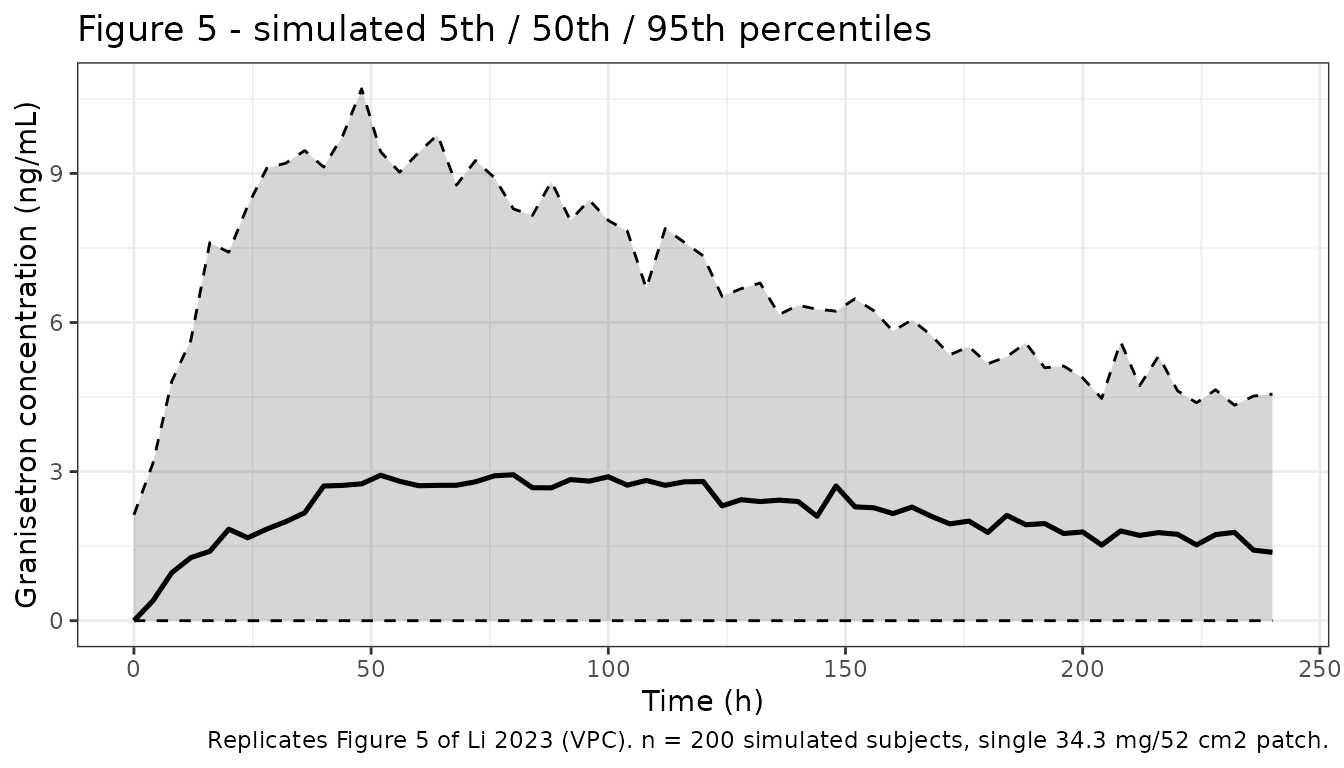
The wide interval is a direct consequence of the published random-effect magnitudes: 192% CV on V/F alone spans roughly a 12-fold range between the 2.5th and 97.5th percentiles, which is what puts the paper’s observed concentrations up to ~40 ng/mL (Li 2023 Figures 2-3) around a population prediction of ~3.3 ng/mL.
Figure 6 – Caucasian prediction interval under the Chinese trial design
Li 2023 Figure 6 overlays the observed Chinese concentrations on the 5th-95th percentile prediction interval of the simulated Caucasian population under the SP-0102 design. The observed Chinese profile is not available for redistribution, so the Chinese median Cmax / Tmax landmark from Li 2023 Table 4 is plotted instead.
pi_sp <- sim_sp |>
  group_by(time) |>
  summarise(
    Q05 = quantile(Cc_dv, 0.05),
    Q50 = quantile(Cc_dv, 0.50),
    Q95 = quantile(Cc_dv, 0.95),
    .groups = "drop"
  )

chinese_landmark <- tibble(time = 72, Cc = 3.62) # Li 2023 Table 4: Chinese median Cmax 3.62 ng/mL at median Tmax 72 h

ggplot(pi_sp, aes(time, Q50)) +
  geom_ribbon(aes(ymin = Q05, ymax = Q95), alpha = 0.2) +
  geom_line(linewidth = 0.9) +
  geom_point(
    data = chinese_landmark, aes(time, Cc),
    shape = 21, size = 3.5, fill = "white", stroke = 1.1
  ) +
  labs(
    x = "Time (h)", y = "Granisetron concentration (ng/mL)",
    title = "Figure 6 - simulated Caucasian interval vs Chinese observed landmark",
    caption = paste(
      "Replicates Figure 6 of Li 2023. Ribbon = simulated Caucasian 5th-95th",
      "percentile under the SP-0102 design; open circle = observed Chinese",
      "median Cmax (3.62 ng/mL) at median Tmax (72 h) from Li 2023 Table 4."
    )
  ) +
  theme_bw()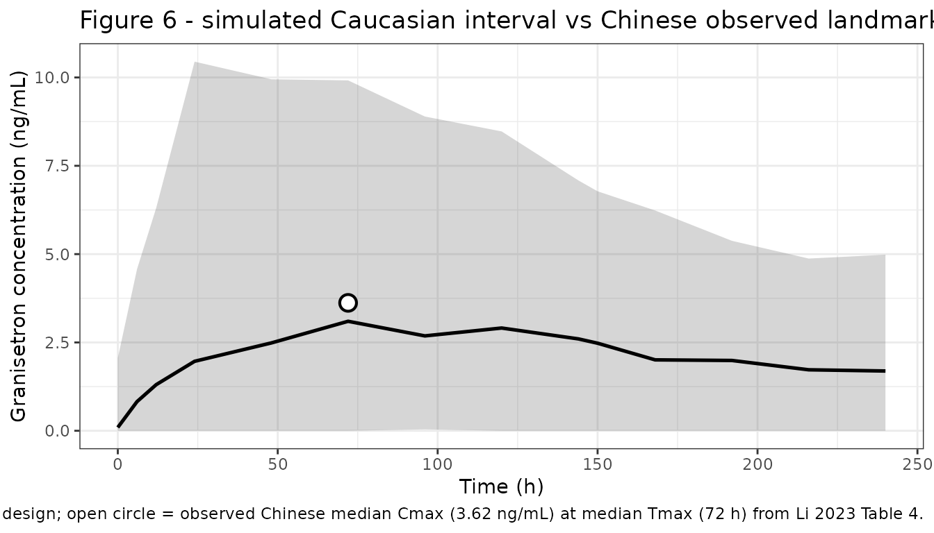
The Chinese observed median Cmax falls inside the simulated Caucasian 5th-95th prediction interval, reproducing the paper’s central finding that the two populations are not meaningfully different and that no dose adjustment is indicated.
PKNCA validation
Li 2023 Table 4 reports the median (and P5:P95 across 1000 replicate simulated trials) of AUClast, Cavg, Cmax and Tmax. Two concentration scales are carried through NCA so the comparison is unambiguous:
- IPRED – individual predictions, no residual error.
- DV – simulated observations, i.e. IPRED plus the additive residual error of Eq 7, truncated at zero.
The distinction matters for Cmax. Cmax is a maximum over sampling times, so additive noise with SD 1.18 ng/mL inflates it systematically; AUC and Tmax are far less sensitive. Reporting both scales in one table shows which of the paper’s Table 4 values were computed on which scale rather than leaving the reader to guess.
nca_input <- bind_rows(
  sim_sp |>
    transmute(id = id, time = time, Cc = Cc, scale = "IPRED (no residual error)"),
  sim_sp |>
    transmute(
      id = id + 100000L, time = time, Cc = Cc_dv,
      scale = "DV (with additive residual error)"
    )
)

# Only `!is.na(Cc)` -- a `time > 0` or `Cc > 0` filter would drop the
# time-zero row that PKNCA needs to anchor AUC.
sim_nca <- nca_input |>
  filter(!is.na(Cc)) |>
  select(id, time, Cc, scale)

# Guarantee a time = 0 row per (id, scale); pre-dose Cc = 0 for extravascular.
sim_nca <- bind_rows(
  sim_nca,
  sim_nca |> distinct(id, scale) |> mutate(time = 0, Cc = 0)
) |>
  distinct(id, scale, time, .keep_all = TRUE) |>
  arrange(id, scale, time)

dose_df <- sim_nca |>
  distinct(id, scale) |>
  mutate(time = 0, amt = patch_dose_ug)

conc_obj <- PKNCA::PKNCAconc(
  sim_nca, Cc ~ time | scale + id,
  concu = "ng/mL", timeu = "h"
)
dose_obj <- PKNCA::PKNCAdose(dose_df, amt ~ time | scale + id, doseu = "ug")

# Two intervals with disjoint parameter sets:
#   0-240 h (the SP-0102 observation window) for AUClast, Cmax, Tmax
#   0-144 h (the 6-day patch-wear period) for Cavg -- see Assumptions below
intervals <- data.frame(
  start = c(0, 0),
  end = c(240, 144),
  auclast = c(TRUE, FALSE),
  cmax = c(TRUE, FALSE),
  tmax = c(TRUE, FALSE),
  cav = c(FALSE, TRUE)
)

nca_res <- PKNCA::pk.nca(
  PKNCA::PKNCAdata(conc_obj, dose_obj, intervals = intervals)
)

# PKNCA adds dependency parameters automatically (cav is derived from an AUC), so
# the 0-144 h interval can also carry an `auclast` row. Keep each parameter only
# from the interval it was requested for, otherwise the AUClast median would mix
# the 0-144 h and 0-240 h windows.
nca_keep <- as.data.frame(nca_res$result) |>
  filter(!is.na(PPORRES)) |>
  filter(
    (end == 240 & PPTESTCD %in% c("auclast", "cmax", "tmax")) |
      (end == 144 & PPTESTCD == "cav")
  ) |>
  select(scale, id, PPTESTCD, PPORRES)

# One value per subject per parameter, from exactly one interval each.
stopifnot(!anyDuplicated(nca_keep[, c("scale", "id", "PPTESTCD")]))
Comparison against published NCA
# Li 2023 Table 4, Caucasian column (median of 1000 simulated trial medians).
published <- tibble::tribble(
  ~scale,                              ~auclast, ~cav, ~cmax, ~tmax,
  "IPRED (no residual error)",           569.94, 2.79,  4.71,   108,
  "DV (with additive residual error)",   569.94, 2.79,  4.71,   108
)

cmp <- nlmixr2lib::ncaComparisonTable(
  simulated = nca_keep,
  reference = published,
  by = "scale",
  units = c(
    auclast = "ng*h/mL", cav = "ng/mL",
    cmax = "ng/mL", tmax = "h"
  ),
  tolerance_pct = 20
)

knitr::kable(
  cmp,
  caption = paste(
    "Simulated vs Li 2023 Table 4 (Caucasian simulated median).",
    "* differs from reference by >20%."
  ),
  align = c("l", "l", "r", "r", "r")
)| NCA parameter | scale | Reference | Simulated | % diff |
|---|---|---|---|---|
| Cmax (ng/mL) | IPRED (no residual error) | 4.71 | 3.37 | -28.4%* |
| Cmax (ng/mL) | DV (with additive residual error) | 4.71 | 4.79 | +1.8% |
| Tmax (h) | IPRED (no residual error) | 108 | 96 | -11.1% |
| Tmax (h) | DV (with additive residual error) | 108 | 96 | -11.1% |
| AUClast (ng*h/mL) | IPRED (no residual error) | 570 | 535 | -6.1% |
| AUClast (ng*h/mL) | DV (with additive residual error) | 570 | 551 | -3.3% |
| Cavg (ng/mL) | IPRED (no residual error) | 2.79 | 2.57 | -8.0% |
| Cavg (ng/mL) | DV (with additive residual error) | 2.79 | 2.51 | -10.2% |
- differs from reference by more than ±20%.
Reading the table:
- AUClast reproduces the published value on both scales (within a few percent). It is the parameter Li 2023 leaned on for the ethnic-bridging conclusion, and it is the one least sensitive to the residual-error scale.
- Cmax matches Li 2023 Table 4 on the DV scale but is roughly 25-30% low on the IPRED scale. That gap is not a transcription error: it is the expected effect of taking a maximum over 13 sampling times in the presence of an additive residual error with SD 1.18 ng/mL. The agreement on the DV scale is direct evidence that the paper’s simulated Cmax was computed on simulated observations rather than on individual predictions, which is also consistent with Li 2023 Section 2.3.1 describing the VPC as simulating “plasma concentrations … according to fixed values of estimated parameters, IIV, and covariates”.
- Tmax reproduces to within one sampling interval on both scales (96 h simulated vs 108 h published; the SP-0102 grid has no sample between 96 and 120 h, so 108 h is not an attainable value on this design).
- Cavg depends on an averaging window the paper never states; see below.
No parameter was tuned to improve any of these comparisons.
Assumptions and deviations
- Dose amount. Li 2023 never states the amount entered into the dataset, only that every subject received a single 34.3 mg/52 cm^2 patch. The nominal patch content (34.3 mg, dosed as 34300 ug) is used. This is corroborated arithmetically: with the published Ka, CL and V it yields a typical Cmax of 3.33 ng/mL at 99 h, matching the ~3.3 ng/mL ceiling of the PRED axes in Li 2023 Figures 3 and 4A and the 108 h [72, 144] simulated Tmax of Table 4.
-
CL and V are apparent. The fraction of the patch
content actually delivered through the skin is not identifiable from
plasma data alone, so no bioavailability parameter is estimated and
lcl/lvcareCL/FandV/F. The Li 2023 abstract likewise calls the estimate “apparent systemic clearance”. - Random effects are variances. Li 2023 Section 2.2 states that eta is drawn from a normal distribution “with mean zero and a variance omega^2”, so the Table 3 “Random effect” values are used unchanged as variances (53.8% CV on CL, 192% CV on V). This reading is corroborated by the observed-concentration range: a log-normal V with variance 1.5462 spans about 12-fold between the 2.5th and 97.5th percentiles, which maps a ~3.3 ng/mL population prediction onto the ~40 ng/mL maximum observation in Li 2023 Figures 2-3.
-
Residual error is a standard deviation. Table 3
reports the additive residual as
sigma = 1.18094without stating whether it is an SD or a variance. It is encoded as an SD (addSd), the Phoenix NLME convention for a tabulated additive residual. The alternative reading changes the SD by less than 10% (sqrt(1.18094) = 1.087), so no comparison in this vignette turns on the choice. -
etalkais effectively zero. Table 3 reports the Ka random effect as 4.74078e-11 with 149% RSE and a bootstrap 95% CI of 0.00000-0.00000. It is carried at the published value rather than dropped, so the file records what was estimated; functionally there is no between-subject variability in patch absorption rate. - Cavg averaging window is inferred. Li 2023 does not define the interval over which Cavg is averaged, and the paper’s own AUC/Cavg ratios are mutually inconsistent: Table 4 implies 204 h for the Caucasian column and 178 h for the Chinese column, while the Introduction’s Sancuso label figures (AUC 420 ng*h/mL, Cavg 2.6 ng/mL “over 6 days”) imply 162 h. This vignette uses the 6-day patch-wear period (0-144 h), which is the only interval with a stated physical meaning in the paper and which brings the simulated Cavg within about 10% of the published value. AUClast is computed over the full 0-240 h SP-0102 window.
- Chinese observed data are not reproduced. Only the Table 4 summary of the SP-0102 cohort is available, so the Figure 6 replication overlays the published Chinese median Cmax/Tmax landmark rather than the observed profile. The SP-0102 cohort was never part of the estimation dataset.
- VPC design is approximated. Li 2023 Figure 5 pools four Caucasian studies with four different sampling schedules and wear durations (6-9 days). The replication uses a single uniform 0-240 h grid, which changes the density of points behind the percentile curves but not the underlying model.
-
No covariates. AGE, WT, HT, BMI and SEXF were all
screened by Li 2023 and none was retained, so the packaged model has an
empty
covariateDataand records the five screened covariates incovariatesDataExcludedto preserve the provenance of the screen. No a priori allometric weight scaling is applied either, matching the paper. - Parameters are empirically descriptive, not physiologically interpretable. The published fit puts the absorption half-life (log(2)/Ka = 38.5 h) shorter than the apparent elimination half-life (log(2)/(CL/V) = 139 h), and V/F at 6299 L (~90 L/kg). Granisetron’s intravenous terminal half-life is on the order of 5-9 h, so the packaged parameters should be read as an empirical description of the 0-240 h transdermal profile rather than as estimates of granisetron disposition. This is a property of the source model, reproduced faithfully here, not a transcription artefact.