Tofacitinib (Tsuchiwata 2026) • nlmixr2lib

Model and source

Citation: Tsuchiwata S, Suzuki A, Wang Q, Kanik K, Fallon L, Menon S. Population pharmacokinetics of tofacitinib in patients with active ankylosing spondylitis. Int J Clin Pharmacol Ther. 2026; 64(2): 57-65. doi:10.5414/CP204781. PMID: 41355395.
Description: One-compartment population PK model with first-order absorption for oral tofacitinib in adults with active ankylosing spondylitis
Article: https://doi.org/10.5414/CP204781
Supplement (goodness-of-fit plots only): https://www.ebi.ac.uk/europepmc/webservices/rest/PMC12825014/supplementaryFiles

Tofacitinib is an oral Janus kinase inhibitor. Tsuchiwata 2026 pooled the tofacitinib arms of a phase 2 dose-ranging study (NCT01786668) and a phase 3 study (NCT03502616) in patients with active ankylosing spondylitis (AS), and described the plasma concentration-time data with a one-compartment disposition model with first-order absorption, parameterised on apparent oral clearance (CL/F), apparent volume of distribution (V/F) and an absorption rate constant (ka).

mod <- readModelDb("Tsuchiwata_2026_tofacitinib")
ui <- rxode2::rxode(mod)
#> ℹ parameter labels from comments will be replaced by 'label()'
ui
#>  ── rxode2-based free-form 2-cmt ODE model ────────────────────────────────────── 
#>  ── Initalization: ──  
#> Fixed Effects ($theta): 
#>              lka              lcl              lvc         e_age_cl 
#>         1.121678         3.299534         4.836282        -0.244000 
#>        e_sexf_cl  e_race_asian_cl   e_crcl_base_cl         e_crp_cl 
#>         0.023700        -0.103000         0.233000        -0.018500 
#>         e_age_vc          e_wt_vc propSd_nontrough    propSd_trough 
#>        -0.230000         0.574000         0.602000         0.696000 
#> 
#> Omega ($omega): 
#>          etalcl   etalvc
#> etalcl 0.079524 0.076000
#> etalvc 0.076000 0.133956
#> attr(,"lotriLabels")
#> [1] NA                                                                           
#> [2] "Table 2, 'IIV (RSE%)' 28.2 and 36.6 and row 'Covariance, CL/F-V/F' = 0.0760"
#> attr(,"lotriFix")
#>        etalcl etalvc
#> etalcl  FALSE  FALSE
#> etalvc  FALSE  FALSE
#> 
#> States ($state or $stateDf): 
#>   Compartment Number Compartment Name
#> 1                  1            depot
#> 2                  2          central
#>  ── μ-referencing ($muRefTable): ──  
#>   theta    eta level covariates
#> 1   lcl etalcl    id           
#> 2   lvc etalvc    id           
#> 
#>  ── Model (Normalized Syntax): ── 
#> function() {
#>     compartmentData <- list(depot = list(analyte = "tofacitinib", 
#>         units = "mg", specimen = "administration site", verified = TRUE), 
#>         central = list(analyte = "tofacitinib", units = "mg", 
#>             specimen = "plasma", verified = TRUE))
#>     covariateData <- list(AGE = list(description = "Baseline age", 
#>         units = "years", type = "continuous", reference_category = NULL, 
#>         notes = "Baseline (time-fixed). Enters CL/F and V/F as separate power functions normalized to the reference value of 40 years (the approximate dataset median; Table 2 footnote b and the reference-patient definition in the Results). Cohort mean 41.8 years (SD 11.7); 64 years is the 95th percentile used for the Figure 2 covariate-impact assessment.", 
#>         source_name = "Age"), SEXF = list(description = "Female sex indicator", 
#>         units = "(binary)", type = "binary", reference_category = "male (SEXF = 0)", 
#>         notes = "Table 2 reports the effect as 'Sex: Female (vs. male)', so male is the reference category and the coefficient is the fractional change in CL/F for a female patient: CL/F is multiplied by (1 + e_sexf_cl * SEXF). The 95% CI of this effect contains the null value; it is retained because the paper reports a full (not reduced) covariate model.", 
#>         source_name = "Sex"), RACE_ASIAN = list(description = "Asian race indicator", 
#>         units = "(binary)", type = "binary", reference_category = "non-Asian (RACE_ASIAN = 0)", 
#>         notes = "Table 2 reports the effect as 'Race: Asian (vs. non-Asian)', a fractional change applied as CL/F * (1 + e_race_asian_cl * RACE_ASIAN). The cohort is 79.9% White, 19.7% Asian and 0.4% not reported (Table 1), so the non-Asian reference group is predominantly White.", 
#>         source_name = "Race"), CRCL_BASE = list(description = "Baseline creatinine clearance (Cockcroft-Gault)", 
#>         units = "mL/min", type = "continuous", reference_category = NULL, 
#>         notes = "Baseline, time-fixed, and NOT body-surface-area normalized -- the paper's BCCL is a raw Cockcroft-Gault creatinine clearance in mL/min, which is why the canonical column is CRCL_BASE rather than the BSA-normalized CRCL. Enters CL/F as a power function normalized to 126 mL/min. Cohort mean 129 mL/min (SD 33.7); the lowest value in the analysis dataset was 48.1 mL/min (Figure 2 footnote a).", 
#>         source_name = "BCCL"), CRP = list(description = "Baseline C-reactive protein", 
#>         units = "mg/dL", type = "continuous", reference_category = NULL, 
#>         notes = "Baseline, time-fixed, standard (not high-sensitivity) assay. UNITS TRAP: this paper reports CRP in mg/dL, not the mg/L used by most other entries in the covariate register -- the reference value 0.851 mg/dL is 8.51 mg/L. Enters CL/F as a power function normalized to 0.851 mg/dL. Cohort mean 1.41 mg/dL (SD 1.55; Table 1). The 95% CI of this effect contains the null value; it is retained because the paper reports a full covariate model.", 
#>         source_name = "BCRP"), WT = list(description = "Baseline body weight", 
#>         units = "kg", type = "continuous", reference_category = NULL, 
#>         notes = "Baseline, time-fixed. Enters V/F only, as a power function normalized to 78 kg (the dataset median). Body weight was pre-specified as a candidate predictor of CL/F as well, but was dropped from the final full model because it correlated with BCCL (r = 0.58) and its inclusion changed the objective function by only -0.066 (Results, Final full model).", 
#>         source_name = "Body weight"))
#>     covariatesDataExcluded <- list(RACE_HISPANIC = list(description = "Hispanic / Latino ethnicity indicator", 
#>         units = "(binary)", type = "binary", notes = "Pre-specified as a candidate predictor of CL/F but not carried into the final full model because 97.8% of the dataset was non-Hispanic/Latino (Results, Final full model development). No coefficient is reported."))
#>     description <- "One-compartment population PK model with first-order absorption for oral tofacitinib in adults with active ankylosing spondylitis"
#>     population <- list(species = "human", n_subjects = 279, n_studies = 2, 
#>         n_observations = 1917, age_mean = "41.8 years (SD 11.7)", 
#>         weight_mean = "78.1 kg (SD 17.4)", weight_median = "78 kg", 
#>         weight_range = "54-107 kg (5th-95th percentiles)", sex_female_pct = 20.4, 
#>         race_ethnicity = c(White = 79.9, Asian = 19.7, NotAvailable = 0.4), 
#>         disease_state = "active ankylosing spondylitis (modified New York criteria, BASDAI >= 4 and BASDAI back-pain score >= 4)", 
#>         dose_range = "2, 5 or 10 mg orally twice daily", renal_function = "baseline Cockcroft-Gault creatinine clearance mean 129 mL/min (SD 33.7); lowest observed 48.1 mL/min", 
#>         regions = "not reported by region; pooled phase 2 (NCT01786668) and phase 3 (NCT03502616) studies", 
#>         notes = "Baseline demographics from Table 1 of Tsuchiwata 2026. Phase 2 (N = 147; 2 mg BID n = 50, 5 mg BID n = 49, 10 mg BID n = 48) and phase 3 (N = 132, all 5 mg BID). Sampling was sparse: week 4 (pre-dose, 0.5 h and 2 h post-dose) and week 8 (pre-dose, 0.5, 2 and 3 h post-dose). Assay range 0.1-100 ng/mL; ~1% of observations were below the limit of quantification and were treated as missing.")
#>     reference <- "Tsuchiwata S, Suzuki A, Wang Q, Kanik K, Fallon L, Menon S. Population pharmacokinetics of tofacitinib in patients with active ankylosing spondylitis. Int J Clin Pharmacol Ther. 2026; 64(2): 57-65. doi:10.5414/CP204781. PMID: 41355395."
#>     units <- list(time = "h", dosing = "mg", concentration = "ng/mL")
#>     vignette <- "Tsuchiwata_2026_tofacitinib"
#>     ini({
#>         lka <- 1.12167756159911
#>         label("Absorption rate constant (1/h)")
#>         lcl <- 3.29953372788566
#>         label("Apparent oral clearance (L/h)")
#>         lvc <- 4.83628190695148
#>         label("Apparent volume of distribution (L)")
#>         e_age_cl <- -0.244
#>         label("Power exponent on (AGE/40) for CL/F (unitless)")
#>         e_sexf_cl <- 0.0237
#>         label("Fractional change in CL/F for female vs male (unitless)")
#>         e_race_asian_cl <- -0.103
#>         label("Fractional change in CL/F for Asian vs non-Asian (unitless)")
#>         e_crcl_base_cl <- 0.233
#>         label("Power exponent on (CRCL_BASE/126) for CL/F (unitless)")
#>         e_crp_cl <- -0.0185
#>         label("Power exponent on (CRP/0.851) for CL/F (unitless)")
#>         e_age_vc <- -0.23
#>         label("Power exponent on (AGE/40) for V/F (unitless)")
#>         e_wt_vc <- 0.574
#>         label("Power exponent on (WT/78) for V/F (unitless)")
#>         propSd_nontrough <- 0.602
#>         label("Proportional residual error SD, time after dose < 9 h (fraction)")
#>         propSd_trough <- 0.696
#>         label("Proportional residual error SD, time after dose >= 9 h (fraction)")
#>         etalcl ~ 0.079524
#>         etalvc ~ c(0.076, 0.133956)
#>         label("Table 2, 'IIV (RSE%)' 28.2 and 36.6 and row 'Covariance, CL/F-V/F' = 0.0760")
#>     })
#>     model({
#>         cov_cl <- (AGE/40)^e_age_cl * (CRCL_BASE/126)^e_crcl_base_cl * 
#>             (CRP/0.851)^e_crp_cl * (1 + e_sexf_cl * SEXF) * (1 + 
#>             e_race_asian_cl * RACE_ASIAN)
#>         cov_vc <- (AGE/40)^e_age_vc * (WT/78)^e_wt_vc
#>         ka <- exp(lka)
#>         cl <- exp(lcl + etalcl) * cov_cl
#>         vc <- exp(lvc + etalvc) * cov_vc
#>         kel <- cl/vc
#>         d/dt(depot) <- -ka * depot
#>         d/dt(central) <- ka * depot - kel * central
#>         Cc <- 1000 * central/vc
#>         trough_flag <- tad() >= 9
#>         propSdTad <- propSd_trough * trough_flag + propSd_nontrough * 
#>             (1 - trough_flag)
#>         Cc ~ prop(propSdTad)
#>     })
#> }

Population

The analysis dataset held 1,917 tofacitinib plasma concentrations from 279 patients (Table 1 and Results, Patient demographics of Tsuchiwata 2026): 147 from the phase 2 study (2 mg BID n = 50, 5 mg BID n = 49, 10 mg BID n = 48) and 132 from the phase 3 study (all 5 mg BID). Patients were 20.4% female, 79.9% White and 19.7% Asian, with a mean body weight of 78.1 kg (SD 17.4), mean age 41.8 years (SD 11.7), mean baseline Cockcroft-Gault creatinine clearance (BCCL) of 129 mL/min (SD 33.7), and mean baseline C-reactive protein (BCRP) of 1.41 mg/dL (SD 1.55).

Sampling was sparse: week 4 (pre-dose, plus 0.5 h and 2 h post-dose) and week 8 (pre-dose, plus 0.5, 2 and 3 h post-dose). The assay range for AS samples was 0.1-100 ng/mL, and about 1% of records were below the limit of quantification and treated as missing.

The same information is available programmatically from the model’s population metadata:

str(ui$population)
#> List of 15
#>  $ species       : chr "human"
#>  $ n_subjects    : num 279
#>  $ n_studies     : num 2
#>  $ n_observations: num 1917
#>  $ age_mean      : chr "41.8 years (SD 11.7)"
#>  $ weight_mean   : chr "78.1 kg (SD 17.4)"
#>  $ weight_median : chr "78 kg"
#>  $ weight_range  : chr "54-107 kg (5th-95th percentiles)"
#>  $ sex_female_pct: num 20.4
#>  $ race_ethnicity: Named num [1:3] 79.9 19.7 0.4
#>   ..- attr(*, "names")= chr [1:3] "White" "Asian" "NotAvailable"
#>  $ disease_state : chr "active ankylosing spondylitis (modified New York criteria, BASDAI >= 4 and BASDAI back-pain score >= 4)"
#>  $ dose_range    : chr "2, 5 or 10 mg orally twice daily"
#>  $ renal_function: chr "baseline Cockcroft-Gault creatinine clearance mean 129 mL/min (SD 33.7); lowest observed 48.1 mL/min"
#>  $ regions       : chr "not reported by region; pooled phase 2 (NCT01786668) and phase 3 (NCT03502616) studies"
#>  $ notes         : chr "Baseline demographics from Table 1 of Tsuchiwata 2026. Phase 2 (N = 147; 2 mg BID n = 50, 5 mg BID n = 49, 10 m"| __truncated__

Source trace

The per-parameter origin is recorded as an in-file comment next to each ini() entry in inst/modeldb/specificDrugs/Tsuchiwata_2026_tofacitinib.R. The table below collects them in one place for review. Every value comes from the main article; the open-access supplement contains only goodness-of-fit plots (Figure S1) and no parameter values.

Equation / parameter	Value	Source location
`lka`	ka = 3.07 1/h	Table 2, row `K a /hour -1` (RSE 10.2%)
`lcl`	CL/F = 27.1 L/h	Table 2, row `CL/F, L/hour` (RSE 2.41%)
`lvc`	V/F = 126 L	Table 2, row `V/F, L` (RSE 2.81%)
`e_age_cl`	-0.244	Table 2, covariate block, CL/F ~ Age
`e_sexf_cl`	0.0237	Table 2, covariate block, CL/F ~ Sex: Female (vs. male)
`e_race_asian_cl`	-0.103	Table 2, covariate block, CL/F ~ Race: Asian (vs. non-Asian)
`e_crcl_base_cl`	0.233	Table 2, covariate block, CL/F ~ BCCL
`e_crp_cl`	-0.0185	Table 2, covariate block, CL/F ~ BCRP
`e_age_vc`	-0.230	Table 2, covariate block, V/F ~ Age
`e_wt_vc`	0.574	Table 2, covariate block, V/F ~ Body weight
`etalcl` variance	0.282^2	Table 2, `IIV (RSE%)` for CL/F = 28.2 (percent CV)
`etalvc` variance	0.366^2	Table 2, `IIV (RSE%)` for V/F = 36.6 (percent CV)
`etalcl`-`etalvc` covariance	0.0760	Table 2, row `Covariance, CL/F-V/F`
`propSd_nontrough`	0.602	Table 2, row `Proportional error CV, TAD < 9 hours,%` = 60.2
`propSd_trough`	0.696	Table 2, row `Proportional error CV, TAD >= 9 hours,%` = 69.6
Reference patient (40 y, male, White, 78 kg, BCCL 126 mL/min, BCRP 0.851 mg/dL)	n/a	Table 2 footnote b; Results, Final full model
Covariate form (power for continuous, one fractional coefficient per category for categorical)	n/a	Table 2 footnote b; Methods, Final full model development
Residual-error split at 9 h after dose	n/a	Methods, Base structural model and random-effects model development
One-compartment disposition, first-order absorption	n/a	Methods, Base structural model; Results, Base structural model

Structural check: steady-state mass balance and half-life

For a linear one-compartment model the steady-state AUC over a dosing interval must equal Dose / (CL/F) exactly. Both sides of this check use the same drawn parameters, so the only difference is numerical integration error and a tight bound is the right assertion.

REF_COV <- list(AGE = 40, SEXF = 0, RACE_ASIAN = 0,
                CRCL_BASE = 126, CRP = 0.851, WT = 78)

# Steady-state observation grid over the final dosing interval: dense through
# absorption and the peak, coarser through the mono-exponential tail.
SS_START <- 156   # time of the 14th (final) q12h dose
TAU <- 12
obs_grid <- function(fine = 0.005, coarse = 0.05) {
  c(seq(SS_START, SS_START + 4, by = fine),
    seq(SS_START + 4 + coarse, SS_START + TAU, by = coarse))
}

# Build a dosing + observation event table for a data frame of subjects.
# `subjects` must carry `id`, `amt` and one column per model covariate.
make_events <- function(subjects, times) {
  ev <- rxode2::et(amt = 1, cmt = "depot", ii = TAU, addl = 13, id = subjects$id) |>
    rxode2::et(times, cmt = "central", id = subjects$id) |>
    as.data.frame()
  ev <- merge(ev, subjects, by = "id", all.x = TRUE)
  ev$amt <- ifelse(ev$evid == 1, ev$dose, ev$amt)
  ev[order(ev$id, ev$time, -ev$evid), ]
}

# The seven covariate scenarios assessed in Tsuchiwata 2026 (Methods and
# Results, "Impact of covariates in the tofacitinib population PK model"),
# plus the reference patient. All use 5 mg BID; for a linear model the
# exposure RATIOS are dose-independent.
scenarios <- tibble::tribble(
  ~scenario,          ~AGE, ~SEXF, ~RACE_ASIAN, ~CRCL_BASE,  ~CRP,  ~WT,
  "Reference",          40,     0,           0,        126, 0.851,   78,
  "Female",             40,     1,           0,        126, 0.851,   78,
  "BWT = 54 kg",        40,     0,           0,        126, 0.851,   54,
  "BWT = 107 kg",       40,     0,           0,        126, 0.851,  107,
  "Age = 64 years",     64,     0,           0,        126, 0.851,   78,
  "BCCL = 50 mL/min",   40,     0,           0,         50, 0.851,   78,
  "BCRP = 8 mg/dL",     40,     0,           0,        126, 8.000,   78,
  "Asian",              40,     0,           1,        126, 0.851,   78
) |>
  mutate(id = row_number(), dose = 5)

ev_scen <- make_events(scenarios, obs_grid(fine = 0.005))

# zeroRe() removes the between-subject variability so each row is the typical
# prediction for that covariate set, which is what the paper's covariate-impact
# assessment reports.
sim_scen <- rxode2::rxSolve(rxode2::zeroRe(mod), events = ev_scen,
                            keep = "id", returnType = "data.frame") |>
  filter(!is.na(Cc), time >= SS_START)
#> ℹ parameter labels from comments will be replaced by 'label()'
#> Warning: No sigma parameters in the model
#> Warning: 'keep' contains id
#> which are output when needed, ignoring these items
#> ℹ omega/sigma items treated as zero: 'etalcl', 'etalvc'
#> Warning: multi-subject simulation without without 'omega'

mb <- sim_scen |>
  group_by(id) |>
  summarise(cl = first(cl), vc = first(vc), dose = 5,
            auc_solved = sum(diff(time) * (head(Cc, -1) + tail(Cc, -1)) / 2),
            .groups = "drop") |>
  mutate(auc_closed = dose * 1000 / cl,           # mg -> ng, so AUC is ng*h/mL
         rel_err = auc_solved / auc_closed - 1,
         thalf = log(2) * vc / cl) |>
  left_join(scenarios |> select(id, scenario), by = "id")

knitr::kable(
  mb |>
    select(scenario, cl, vc, auc_closed, auc_solved, rel_err, thalf) |>
    dplyr::rename("Scenario" = scenario, "CL/F (L/h)" = cl, "V/F (L)" = vc,
                  "Dose/(CL/F) (ng*h/mL)" = auc_closed,
                  "Solved AUC0-tau (ng*h/mL)" = auc_solved,
                  "Relative error" = rel_err, "t1/2 (h)" = thalf),
  digits = c(0, 3, 2, 2, 2, 8, 3),
  caption = "Steady-state mass balance: solved AUC over the dosing interval vs the closed form Dose/(CL/F)."
)

Steady-state mass balance: solved AUC over the dosing interval vs the closed form Dose/(CL/F).
Scenario	CL/F (L/h)	V/F (L)	Dose/(CL/F) (ng*h/mL)	Solved AUC0-tau (ng*h/mL)	Relative error	t1/2 (h)
Reference	27.100	126.00	184.50	184.50	2.47e-06	3.223
Female	27.742	126.00	180.23	180.23	2.57e-06	3.148
BWT = 54 kg	27.100	102.02	184.50	184.50	3.35e-06	2.610
BWT = 107 kg	27.100	151.07	184.50	184.50	1.80e-06	3.864
Age = 64 years	24.164	113.09	206.92	206.92	2.45e-06	3.244
BCCL = 50 mL/min	21.850	126.00	228.84	228.84	1.69e-06	3.997
BCRP = 8 mg/dL	26.000	126.00	192.31	192.31	2.31e-06	3.359
Asian	24.309	126.00	205.69	205.69	2.06e-06	3.593


stopifnot(
  # Deterministic: same parameters on both sides, so the residual is pure
  # trapezoidal-integration error. Realised max 3e-6 on the grid above.
  max(abs(mb$rel_err)) < 1e-4,
  # Table 2 footnote: "The derived elimination half-life was ~ 3 hours."
  # Reference patient: log(2) * 126 / 27.1 = 3.22 h.
  abs(mb$thalf[mb$scenario == "Reference"] - 3.22) < 0.02
)

Covariate model: reproducing the published effect sizes

Tsuchiwata 2026 states each covariate’s effect on CL/F and V/F as a percent change relative to the reference patient (Results, Impact of covariates in the tofacitinib population PK model). Those eight printed numbers over-determine the covariate model: reproducing all of them confirms the functional form (power for continuous covariates normalised to the reference value; a single fractional coefficient per category for categorical covariates), the reference values (40 years, 78 kg, 126 mL/min, 0.851 mg/dL) and the sign of every coefficient.

ref <- mb |> filter(scenario == "Reference")

published_effects <- tibble::tribble(
  ~scenario,          ~parameter, ~published_pct,
  "Age = 64 years",   "CL/F",            -10.9,
  "Female",           "CL/F",              2.4,
  "Asian",            "CL/F",            -10.3,
  "BCCL = 50 mL/min", "CL/F",            -19.4,
  "BCRP = 8 mg/dL",   "CL/F",             -4.1,
  "Age = 64 years",   "V/F",             -10.2,
  "BWT = 54 kg",      "V/F",             -19.0,
  "BWT = 107 kg",     "V/F",              20.0
)

cov_effects <- mb |>
  transmute(scenario,
            `CL/F` = 100 * (cl / ref$cl - 1),
            `V/F`  = 100 * (vc / ref$vc - 1)) |>
  pivot_longer(c(`CL/F`, `V/F`), names_to = "parameter", values_to = "model_pct") |>
  inner_join(published_effects, by = c("scenario", "parameter")) |>
  mutate(abs_diff = abs(model_pct - published_pct))

knitr::kable(
  cov_effects |>
    dplyr::rename("Scenario" = scenario, "Parameter" = parameter,
                  "Model (% change)" = model_pct,
                  "Published (% change)" = published_pct,
                  "|difference| (percentage points)" = abs_diff),
  digits = 3,
  caption = "Percent change in CL/F and V/F vs the reference patient, model vs Tsuchiwata 2026 Results."
)

Percent change in CL/F and V/F vs the reference patient, model vs Tsuchiwata 2026 Results.
Scenario	Parameter	Model (% change)	Published (% change)	\|difference\| (percentage points)
Female	CL/F	2.370	2.4	0.030
BWT = 54 kg	V/F	-19.029	-19.0	0.029
BWT = 107 kg	V/F	19.896	20.0	0.104
Age = 64 years	CL/F	-10.835	-10.9	0.065
Age = 64 years	V/F	-10.246	-10.2	0.046
BCCL = 50 mL/min	CL/F	-19.374	-19.4	0.026
BCRP = 8 mg/dL	CL/F	-4.061	-4.1	0.039
Asian	CL/F	-10.300	-10.3	0.000


stopifnot(
  # Deterministic algebra on both sides. The residual is the paper rounding
  # each coefficient to three significant figures: the largest gap is the
  # 107 kg V/F effect (19.90% computed vs "20%" printed, 0.10 percentage
  # points). 0.2 leaves headroom for that rounding and still goes red on a
  # transposed exponent, a wrong reference value or a sign error, all of
  # which move these numbers by whole percentage points or flip them.
  max(cov_effects$abs_diff) < 0.2
)

Replicating Figure 2: covariate impact on AUC and Cmax

Figure 2 of Tsuchiwata 2026 is a forest plot of steady-state AUC and Cmax ratios relative to the typical subject. The abstract states the printed summary of that figure: excluding BCCL, the AUC point estimates ranged from 98 to 112% and the Cmax point estimates from 89 to 115%; for BCCL = 50 mL/min the AUC was 24% higher than the reference.

NCA is computed with PKNCA over the final dosing interval, with the time axis shifted so the last dose sits at t = 0.

nca_frame <- function(sim, group_col) {
  out <- sim |>
    filter(!is.na(Cc)) |>
    transmute(id, time = time - SS_START, Cc,
              grp = as.character(.data[[group_col]]))
  # Guarantee a record at the interval start (extravascular pre-dose Cc = 0).
  bind_rows(out, out |> distinct(id, grp) |> mutate(time = 0, Cc = 0)) |>
    distinct(id, grp, time, .keep_all = TRUE) |>
    arrange(id, grp, time)
}

conc_scen <- sim_scen |>
  left_join(scenarios |> select(id, scenario), by = "id") |>
  nca_frame("scenario")

dose_scen <- scenarios |> transmute(id, grp = scenario, time = 0, amt = dose)

nca_scen <- PKNCA::pk.nca(PKNCA::PKNCAdata(
  PKNCA::PKNCAconc(as.data.frame(conc_scen), Cc ~ time | grp + id,
                   concu = "ng/mL", timeu = "h"),
  PKNCA::PKNCAdose(as.data.frame(dose_scen), amt ~ time | grp + id,
                   doseu = "mg"),
  intervals = data.frame(start = 0, end = TAU,
                         cmax = TRUE, tmax = TRUE, auclast = TRUE,
                         half.life = TRUE)
))

# Replicates Figure 2 of Tsuchiwata 2026: AUC and Cmax ratios relative to the
# typical (reference) subject. Point estimates only -- the paper's 90% CIs come
# from 1,000 nonparametric bootstrap replicates that are not published.
ratios <- as.data.frame(nca_scen$result) |>
  filter(PPTESTCD %in% c("cmax", "auclast")) |>
  select(scenario = grp, PPTESTCD, PPORRES) |>
  pivot_wider(names_from = PPTESTCD, values_from = PPORRES)

ref_r <- ratios |> filter(scenario == "Reference")
ratios <- ratios |>
  mutate(AUC = 100 * auclast / ref_r$auclast,
         Cmax = 100 * cmax / ref_r$cmax) |>
  filter(scenario != "Reference")

fig2 <- ratios |>
  select(scenario, AUC, Cmax) |>
  pivot_longer(c(AUC, Cmax), names_to = "metric", values_to = "ratio") |>
  mutate(scenario = factor(scenario, levels = rev(c(
    "Female", "BWT = 54 kg", "BWT = 107 kg", "Age = 64 years",
    "BCCL = 50 mL/min", "BCRP = 8 mg/dL", "Asian"))),
    metric = factor(metric, levels = c("Cmax", "AUC")))

ggplot(fig2, aes(x = ratio, y = scenario, shape = metric)) +
  geom_vline(xintercept = c(80, 100, 125), linetype = "dashed") +
  geom_point(size = 2.5, position = position_dodge(width = 0.55)) +
  scale_x_continuous(limits = c(60, 150), breaks = c(60, 80, 100, 125, 150)) +
  labs(x = "Change relative to the typical subject (%)", y = NULL,
       shape = NULL,
       title = "Figure 2 -- covariate impact on steady-state exposure",
       caption = "Replicates Figure 2 of Tsuchiwata 2026 (point estimates only).") +
  theme_bw()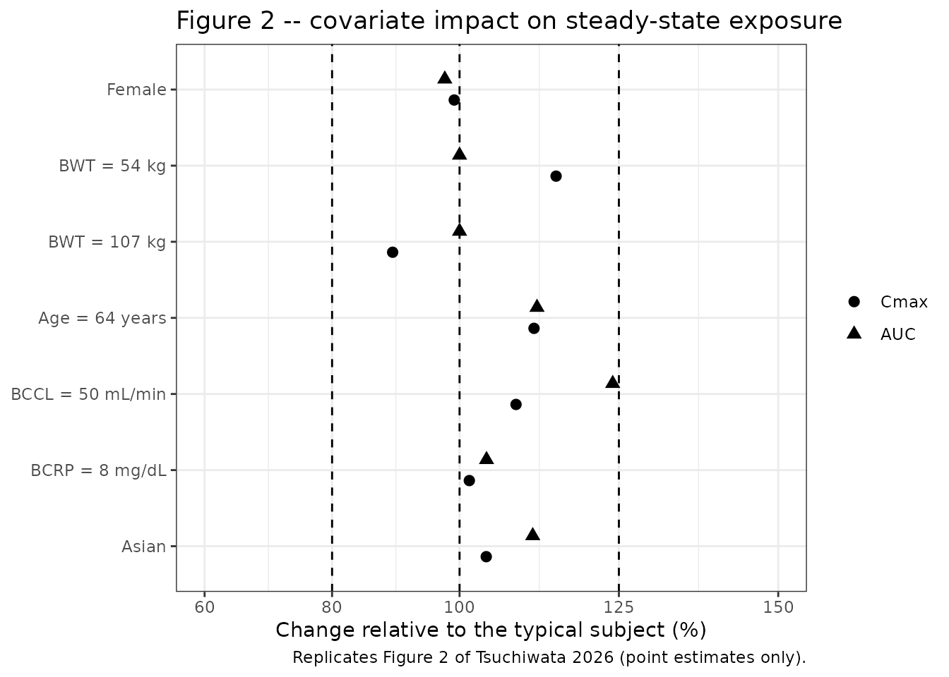

excl_bccl <- ratios |> filter(!scenario %in% c("BCCL = 50 mL/min", "BCRP = 8 mg/dL"))

fig2_claims <- tibble::tribble(
  ~claim,                                                 ~published, ~model,
  "Lowest AUC ratio excluding BCCL (%)",                          98, min(excl_bccl$AUC),
  "Highest AUC ratio excluding BCCL (%)",                        112, max(excl_bccl$AUC),
  "Lowest Cmax ratio excluding BCCL (%)",                         89, min(excl_bccl$Cmax),
  "Highest Cmax ratio excluding BCCL (%)",                       115, max(excl_bccl$Cmax),
  "AUC ratio at BCCL = 50 mL/min (%)",                           124,
    ratios$AUC[ratios$scenario == "BCCL = 50 mL/min"]
) |>
  mutate(abs_diff = abs(model - published))

knitr::kable(
  fig2_claims |>
    dplyr::rename("Published claim" = claim, "Published" = published,
                  "Model" = model, "|difference| (percentage points)" = abs_diff),
  digits = 2,
  caption = "Abstract-level exposure-ratio claims of Tsuchiwata 2026 vs the packaged model."
)

Abstract-level exposure-ratio claims of Tsuchiwata 2026 vs the packaged model.
Published claim	Published	Model	\|difference\| (percentage points)
Lowest AUC ratio excluding BCCL (%)	98	97.68	0.32
Highest AUC ratio excluding BCCL (%)	112	112.15	0.15
Lowest Cmax ratio excluding BCCL (%)	89	89.50	0.50
Highest Cmax ratio excluding BCCL (%)	115	115.15	0.15
AUC ratio at BCCL = 50 mL/min (%)	124	124.03	0.03


stopifnot(
  # Deterministic (typical-value) quantities on both sides. The residual is
  # the paper reporting integer percentages: the largest gap is the 89.50%
  # Cmax minimum printed as "89". 1.0 percentage point covers that and still
  # goes red on any covariate mis-transcription.
  max(fig2_claims$abs_diff) < 1.0
)

Virtual cohort

Original subject-level data are not public. The cohort below reproduces the Table 1 marginal distributions: body weight (mean 78.1 kg, SD 17.4), age (mean 41.8 years, SD 11.7), BCCL (mean 129 mL/min, SD 33.7), 20.4% female and 19.7% Asian. Body weight and BCCL are drawn jointly with the correlation of 0.58 that the paper reports between them (Results, Final full model). BCRP is drawn log-normally to match its mean of 1.41 mg/dL and SD of 1.55 mg/dL, which are too dispersed for a normal distribution.

# set.seed() seeds R's RNG for the covariate draw. It does NOT seed rxode2's
# simulation RNG, whose streams are partitioned per solver thread -- so the
# etas drawn below differ between a 16-thread workstation and a 2-core CI
# runner. Every assertion downstream is written to hold for any cohort the
# model can produce; see the bounds' comments.
set.seed(20260910)
rxode2::rxSetSeed(20260910)

N_PER_ARM <- 200   # skill cap: never more than 200 participants per arm

make_cohort <- function(dose, id_offset) {
  z <- matrix(rnorm(2 * N_PER_ARM), ncol = 2) %*%
    chol(matrix(c(1, 0.58, 0.58, 1), nrow = 2))
  crp_sd <- sqrt(log(1 + (1.55 / 1.41)^2))
  tibble(
    id = id_offset + seq_len(N_PER_ARM),
    AGE = pmin(pmax(rnorm(N_PER_ARM, 41.8, 11.7), 18), 80),
    WT = pmin(pmax(78.1 + 17.4 * z[, 1], 40), 160),
    # 48.1 mL/min was the lowest BCCL in the analysis dataset (Figure 2 note a).
    CRCL_BASE = pmin(pmax(129 + 33.7 * z[, 2], 48.1), 260),
    SEXF = rbinom(N_PER_ARM, 1, 0.204),
    RACE_ASIAN = rbinom(N_PER_ARM, 1, 0.197),
    CRP = pmin(rlnorm(N_PER_ARM, log(1.41) - crp_sd^2 / 2, crp_sd), 20),
    dose = dose,
    treatment = paste0(dose, " mg BID")
  )
}

cohort <- bind_rows(
  make_cohort(2, 0L),
  make_cohort(5, 1000L),
  make_cohort(10, 2000L)
) |>
  mutate(treatment = factor(treatment,
                            levels = c("2 mg BID", "5 mg BID", "10 mg BID")))

events <- make_events(cohort, obs_grid(fine = 0.05, coarse = 0.25))
stopifnot(!anyDuplicated(unique(events[, c("id", "time", "evid")])))

Simulation

sim <- rxode2::rxSolve(mod, events = events,
                       keep = c("treatment", "dose"),
                       returnType = "data.frame") |>
  filter(!is.na(Cc), time >= SS_START) |>
  mutate(treatment = factor(as.character(treatment),
                            levels = c("2 mg BID", "5 mg BID", "10 mg BID")))
#> ℹ parameter labels from comments will be replaced by 'label()'

stopifnot(all(sim$Cc >= 0), !anyNA(sim$Cc))

Replicating Figure 1: steady-state concentration-time profiles

Figure 1 of Tsuchiwata 2026 is a visual predictive check stratified by dose group, shown over 24 hours (panel A) and over the first 4 hours (panel B), with the 5th, 50th and 95th percentiles. The panels below plot the same percentiles from the packaged model over one steady-state dosing interval. Cc carries no residual error, so these are model predictions rather than a full VPC of simulated observations.

vpc <- sim |>
  mutate(tad = time - SS_START) |>
  group_by(treatment, tad) |>
  summarise(Q05 = quantile(Cc, 0.05), Q50 = median(Cc),
            Q95 = quantile(Cc, 0.95), .groups = "drop")

ggplot(vpc, aes(tad, Q50)) +
  geom_ribbon(aes(ymin = Q05, ymax = Q95), alpha = 0.25) +
  geom_line() +
  facet_wrap(~treatment) +
  labs(x = "Time after dose (h)", y = "Tofacitinib concentration (ng/mL)",
       title = "Figure 1A -- steady-state profile by dose group",
       caption = "Replicates Figure 1 of Tsuchiwata 2026 (median with 5th-95th percentile band).") +
  theme_bw()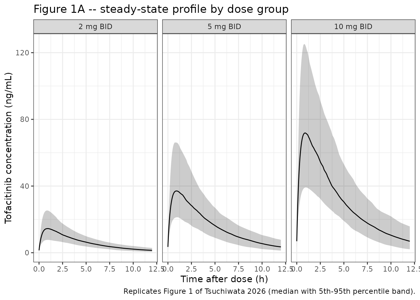


ggplot(filter(vpc, tad <= 4), aes(tad, Q50)) +
  geom_ribbon(aes(ymin = Q05, ymax = Q95), alpha = 0.25) +
  geom_line() +
  facet_wrap(~treatment) +
  labs(x = "Time after dose (h)", y = "Tofacitinib concentration (ng/mL)",
       title = "Figure 1B -- first 4 hours after dose",
       caption = "Replicates Figure 1B of Tsuchiwata 2026.") +
  theme_bw()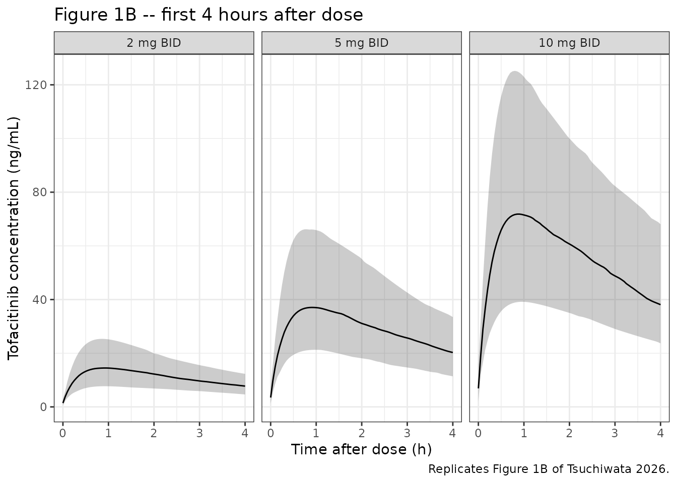

PKNCA validation

conc_pop <- nca_frame(sim, "treatment")
dose_pop <- cohort |> transmute(id, grp = as.character(treatment), time = 0, amt = dose)

nca_res <- PKNCA::pk.nca(PKNCA::PKNCAdata(
  PKNCA::PKNCAconc(as.data.frame(conc_pop), Cc ~ time | grp + id,
                   concu = "ng/mL", timeu = "h"),
  PKNCA::PKNCAdose(as.data.frame(dose_pop), amt ~ time | grp + id,
                   doseu = "mg"),
  intervals = data.frame(start = 0, end = TAU,
                         cmax = TRUE, tmax = TRUE, auclast = TRUE,
                         cav = TRUE, clast.obs = TRUE, half.life = TRUE)
))

Comparison against published exposures

Tsuchiwata 2026 reports geometric mean (%CV) steady-state AUC and Cmax by dose group (Results, Impact of covariates). Those exposures were “generated using the individual parameters obtained using the population PK model”, so the comparison below uses the model prediction Cc rather than a residual-error-perturbed observation, and aggregates with the geometric mean to match the published statistic.

geomean <- function(x) exp(mean(log(x)))

sim_gm <- as.data.frame(nca_res$result) |>
  filter(PPTESTCD %in% c("cmax", "auclast", "half.life"), !is.na(PPORRES)) |>
  group_by(treatment = grp, PPTESTCD) |>
  summarise(PPORRES = geomean(PPORRES), .groups = "drop")

published <- tibble::tribble(
  ~treatment,   ~cmax, ~auclast, ~half.life,
  "2 mg BID",    14.0,     72.2,       3.22,
  "5 mg BID",    36.7,    191.0,       3.22,
  "10 mg BID",   73.9,    372.0,       3.22
)

cmp <- nlmixr2lib::ncaComparisonTable(
  simulated = sim_gm,
  reference = published,
  by = "treatment",
  units = c(cmax = "ng/mL", auclast = "ng*h/mL", half.life = "h"),
  tolerance_pct = 20
)

knitr::kable(
  cmp,
  caption = paste(
    "Simulated (geometric mean over the virtual cohort) vs published",
    "steady-state exposures. AUC0-tau and Cmax are the geometric means of",
    "Tsuchiwata 2026 Results; the half-life reference is the derived value",
    "log(2) * 126 / 27.1 = 3.22 h behind the paper's '~ 3 hours' footnote.",
    "* marks a difference above 20%."
  ),
  align = c("l", "l", "r", "r", "r")
)

Simulated (geometric mean over the virtual cohort) vs published steady-state exposures. AUC0-tau and Cmax are the geometric means of Tsuchiwata 2026 Results; the half-life reference is the derived value log(2) * 126 / 27.1 = 3.22 h behind the paper’s ‘~ 3 hours’ footnote. * marks a difference above 20%.
NCA parameter	treatment	Reference	Simulated	% diff
Cmax (ng/mL)	2 mg BID	14	14.1	+1.0%
Cmax (ng/mL)	5 mg BID	36.7	36.7	-0.1%
Cmax (ng/mL)	10 mg BID	73.9	71.9	-2.7%
AUClast (ng*h/mL)	2 mg BID	72.2	74	+2.5%
AUClast (ng*h/mL)	5 mg BID	191	188	-1.4%
AUClast (ng*h/mL)	10 mg BID	372	372	+0.0%
t½ (h)	2 mg BID	3.22	3.3	+2.6%
t½ (h)	5 mg BID	3.22	3.21	-0.4%
t½ (h)	10 mg BID	3.22	3.25	+0.8%

gm_pct <- as.data.frame(nca_res$result) |>
  filter(PPTESTCD %in% c("cmax", "auclast"), !is.na(PPORRES)) |>
  group_by(treatment = grp, PPTESTCD) |>
  summarise(sim = geomean(PPORRES), .groups = "drop") |>
  left_join(published |> pivot_longer(c(cmax, auclast), names_to = "PPTESTCD",
                                      values_to = "ref"),
            by = c("treatment", "PPTESTCD")) |>
  mutate(pct = 100 * (sim / ref - 1))

stopifnot(
  # Cohort-derived, so the bound must hold for ANY cohort the model can draw,
  # not just this one. Realised max |% diff| was 4.80 / 2.68 / 3.00 / 2.75 at
  # 1 / 2 / 4 / 16 solver threads; 12 sits well outside that spread and still
  # goes red on a mis-transcribed clearance, dose or unit, which move these
  # geometric means by tens of percent or more.
  max(abs(gm_pct$pct)) < 12,
  # Dose proportionality: AUC per mg must be flat across the three arms for a
  # linear model. Deterministic in expectation but cohort-dependent, so this is
  # a magnitude bound, not an equality.
  {
    per_mg <- gm_pct |> filter(PPTESTCD == "auclast") |>
      mutate(dose = as.numeric(sub(" mg BID", "", treatment)), per_mg = sim / dose)
    max(per_mg$per_mg) / min(per_mg$per_mg) < 1.15
  }
)

Residual-error structure

The paper used two proportional residual-error models split at 9 hours after dose (60.2% CV for TAD < 9 h and 69.6% CV for TAD >= 9 h). The packaged model assembles that switch inside model() from tad() and passes it to prop(), so the observation sim carries the correct error magnitude on each side of the split. Comparing the spread of sim / Cc either side of 9 h recovers the two published CVs.

sim_err <- rxode2::rxSolve(
  mod,
  events = make_events(make_cohort(5, 5000L), SS_START + c(2, 10)),
  returnType = "data.frame"
) |>
  filter(!is.na(sim)) |>
  mutate(tad = time - SS_START,
         stratum = ifelse(tad >= 9, "TAD >= 9 h", "TAD < 9 h"),
         ratio = sim / Cc)

err_tab <- sim_err |>
  group_by(stratum) |>
  summarise(n = n(), model_cv_pct = 100 * sd(ratio), .groups = "drop") |>
  mutate(published_cv_pct = ifelse(stratum == "TAD >= 9 h", 69.6, 60.2))

knitr::kable(
  err_tab |>
    dplyr::rename("Stratum" = stratum, "n" = n,
                  "Model residual CV (%)" = model_cv_pct,
                  "Published residual CV (%)" = published_cv_pct),
  digits = 1,
  caption = "Proportional residual-error CV recovered from the simulated observations, by time-after-dose stratum."
)

Proportional residual-error CV recovered from the simulated observations, by time-after-dose stratum.
Stratum	n	Model residual CV (%)	Published residual CV (%)
TAD < 9 h	200	61	60.2
TAD >= 9 h	200	66	69.6


stopifnot(
  # A sample SD from n = 200 draws has a relative standard error of about
  # 1/sqrt(2n) = 5%, so ~15 CV points of tolerance is roughly 3 standard
  # errors. The gate still goes red if the two strata are swapped (a 9.4-point
  # gap in the wrong direction) or if the switch is not wired up at all.
  all(abs(err_tab$model_cv_pct - err_tab$published_cv_pct) < 15),
  # The trough stratum must be the more variable one -- that is the whole point
  # of the split, and it is a 9.4-point difference, not a coin flip.
  err_tab$model_cv_pct[err_tab$stratum == "TAD >= 9 h"] >
    err_tab$model_cv_pct[err_tab$stratum == "TAD < 9 h"]
)

Assumptions and deviations

Omega scale. Table 2 labels its variability column IIV (RSE%) and the abbreviation list expands IIV as “inter-individual variance”, but the values (28.2 and 36.6) are percent CVs: the Results text reports the base model’s IIV as “30.5%” and “39.2%” in the same style, and a variance of 0.282 would correspond to a 58% CV, far larger than any tofacitinib population analysis the paper compares against. The variances are therefore encoded as (CV/100)^2, i.e. 0.282^2 and 0.366^2. The off-diagonal is the covariance the paper reports directly on the variance scale (0.0760), giving a correlation of 0.736 and a positive-definite block. The two competing conventions – omega^2 = (CV/100)^2 versus omega^2 = log(CV^2 + 1) – give 0.0795 vs 0.0765 for CL/F and 0.1340 vs 0.1257 for V/F, and nothing printed in the paper discriminates between them; the first was used because it is the standard NONMEM reporting convention (%CV = 100 * sqrt(OMEGA)).
Inter-occasion variability on F is omitted. The Methods state that “inter-occasional variability was taken into consideration in the parameter F”, but no IOV magnitude is reported in Table 2, in the Results text, or in the open-access supplement (which contains only goodness-of-fit plots). No value was invented; the packaged model has no IOV term and F is folded into the apparent parameters CL/F and V/F. Simulated within-subject occasion-to-occasion variability is therefore lower than the original analysis would produce.
Bioavailability is not separately identifiable. The paper reports apparent parameters (CL/F, V/F) from oral data only, so no f(depot) term is encoded and doses enter the depot at face value.
Non-significant covariates are retained. The 95% CIs for the effects of BCRP and female sex on CL/F contain the null value. They are kept because Table 2 is the full covariate model, which is what the paper reports and what this extraction replicates.
Body weight on CL/F and Hispanic ethnicity are not in the model. Both were pre-specified candidates. Body weight was dropped from CL/F because it correlated with BCCL (r = 0.58) and added only -0.066 to the objective function; ethnicity was dropped because 97.8% of the dataset was non-Hispanic/Latino. RACE_HISPANIC is recorded in the model file’s covariatesDataExcluded list to preserve the covariate screen without implying an effect.
CRP units are mg/dL, not mg/L. Most entries in the covariate register carry CRP in mg/L. This paper reports it in mg/dL, and the reference value 0.851 mg/dL equals 8.51 mg/L. A cohort supplied in mg/L would produce a CL/F roughly 4% too low across the board.
BCCL is a raw Cockcroft-Gault creatinine clearance in mL/min, not BSA-normalised, so the canonical covariate column is CRCL_BASE rather than the BSA-normalised CRCL.
Virtual-cohort covariate distributions are assumed. Table 1 gives only means and standard deviations, so normal (age, weight, BCCL) and log-normal (BCRP) marginals were assumed, truncated to physiologically plausible ranges. Weight and BCCL are drawn with the reported correlation of 0.58; age’s correlation with BCCL (-0.412, Results) is not imposed, which slightly overstates the independent spread of CL/F in the cohort.
Simulated %CVs exceed the published ones. The virtual cohort gives AUC %CVs near 28-29% against the published 21.8-25.4%, and Cmax %CVs near 33-34% against 22.5-28.0%. The published values are dispersions of empirical Bayes individual parameters, which are shrunk toward the typical value (reported shrinkage 21.5% on IIV of CL/F and 24.8% on IIV of V/F), whereas the virtual cohort is drawn from the full unshrunk omega and also carries covariate variability. Only the geometric means are gated.
Figure 2 confidence intervals are not reproduced. The paper’s 90% CIs come from 1,000 nonparametric bootstrap replicates whose parameter draws are not published, so the replication plots point estimates only.
Dosing regimen for the exposure comparison. The paper does not state the simulation regimen behind its geometric-mean exposures beyond the dose levels. Fourteen q12h doses (156 h, roughly 48 half-lives) are used here so that the final interval is unambiguously at steady state.