Cancer vaccine + IL-12 tumor immunotherapy in mice (Parra-Guillen 2013)
Source:vignettes/articles/ParraGuillen_2013_tumor_immunotherapy.Rmd
ParraGuillen_2013_tumor_immunotherapy.RmdModel and source
- Citation: Parra-Guillen ZP, Berraondo P, Grenier E, Ribba B, Troconiz IF. Mathematical Model Approach to Describe Tumour Response in Mice After Vaccine Administration and its Applicability to Immune-Stimulatory Cytokine-Based Strategies. The AAPS Journal 2013;15(3):797-807. doi:10.1208/s12248-013-9483-5.
- Description: Preclinical (mouse, female C57BL/6 with subcutaneous TC1 tumor expressing HPV E7). Semi-mechanistic K-PD tumor-growth-dynamics model of single-dose CyaA-E7 cancer vaccine: a virtual vaccine compartment feeds a two-compartment transit chain to a vaccine-elicited inhibitory signal SVAC that reduces tumor size via a second-order k3 * SVAC * tumor_size term, inhibited by a Hill-function regulator REG driven by tumor size; a binary mixture covariate MIX_VAC_RELAPSE gates the SVAC degradation rate (k2 = 0 for cure, k2 = k1 for relapse).
- Article: https://doi.org/10.1208/s12248-013-9483-5
This paper develops a semi-mechanistic K-PD tumor-growth-dynamics model on a preclinical (mouse) CyaA-E7 cancer-vaccine dataset and then re-fits the same structural equations to a separately published IL-12 hydrodynamic-plasmid dataset to demonstrate the model’s applicability to other immune-stimulatory therapies. The package therefore ships two model files that share equations but differ in cohort-specific parameter values:
-
modellib("ParraGuillen_2013_cyaaE7")– the model-build dataset (TC1 tumor in C57BL/6 mice, single IV dose of 50 ug CyaA-E7 vaccine on one of days 4 / 7 / 11 / 18 / 25 / 30). All structural and IAV parameters are estimated. -
modellib("ParraGuillen_2013_il12")– the applicability dataset (MC38 tumor in C57BL/6 mice, single hydrodynamic injection of 10 ug murine-IL-12 plasmid on day 23). Cell-line and immunotherapeutic-kinetics parameters (Ts0, lambda, k1, REG50 + IAV) are re-fit; vaccine-efficacy / regulator parameters (k3, k4, gamma) and the mixture probability P(1) are carried fixed from the CyaA-E7 build.
Both files use the binary covariate MIX_VAC_RELAPSE (1 =
relapser, 0 = cure) to gate the SVAC degradation rate. The Bernoulli
probability of relapse is 1 - P(1) = 0.156, fixed.
Population
The CyaA-E7 model-build cohort comprised 93 female C57BL/6 mice (5 weeks old) inoculated subcutaneously with 5 x 10^5 TC1 cells (a mouse lung-epithelial line transformed with HPV-16 E6 / E7 and activated H-Ras). The arms were PBS day 4 (n = 19), CyaA-E7 50 ug IV day 4 (n = 15), day 7 (n = 16), day 11 (n = 14), day 18 (n = 15), day 25 (n = 14), and day 30 (n = 15). A separate 34-mouse external validation cohort (PBS day 4 n = 23; CyaA-E7 day 25 n = 11) was held out from the fit.
The IL-12 applicability cohort comprised 33 female C57BL/6 mice inoculated subcutaneously with 5 x 10^5 MC38 colon-adenocarcinoma cells. Arms were PBS control (n = 12) and IL-12 plasmid 10 ug hydrodynamic injection on day 23 (n = 21).
Tumor size was reported as the mean of two perpendicular diameters; 2
mm was the limit of quantification (61.6 % of observations were BQL and
treated as censored using the NONMEM Laplacian M3 likelihood).
Population information is also available programmatically via
readModelDb("ParraGuillen_2013_cyaaE7")$population and
readModelDb("ParraGuillen_2013_il12")$population.
Mathematical model
The five-ODE system (Equations 1-5 of the source, page 799):
dVAC/dt        = - k1 * VAC                                       (Eq. 1)
dTRAN/dt       =   k1 * VAC  - k1 * TRAN                          (Eq. 2)
dSVAC/dt       =   k1 * TRAN - k2 * SVAC                          (Eq. 3)
dTs/dt         = lambda - k3 * REG50^gamma / (REG50^gamma + REG^gamma) * Ts * SVAC   (Eq. 4)
dREG/dt        = k4 * Ts - k4 * REG                               (Eq. 5)
Initial conditions at tumor cell inoculation (day 0):
Ts(0) = Ts0, the rest zero. The vaccine virtual compartment
VAC is reset to 1 at the time of vaccine injection (paper
Methods p. 799: “VAC0 was set to an arbitrary value of 1 due to the
absence of pharmacokinetic data”). The mixture covariate
MIX_VAC_RELAPSE gates k2:
-
MIX_VAC_RELAPSE = 0(responder / cure, P(1) = 0.844):k2 = 0, so SVAC remains constant once formed and the tumor is eradicated permanently. -
MIX_VAC_RELAPSE = 1(relapser, 1 - P(1) = 0.156):k2 = k1, so SVAC decays at the same rate as the vaccine virtual drug, and the tumor regrows after vaccine clearance.
The shared k1 between vaccine elimination and SVAC
degradation is forced by identifiability (Methods last paragraph
p. 799).
Source trace
| Equation / parameter | CyaA-E7 value | IL-12 value | Source location |
|---|---|---|---|
Ts0 (initial tumor size) |
0.324 mm | 1.16e-6 mm | Table I row Ts0
|
lambda (zero-order growth) |
0.354 mm / day | 0.335 mm / day | Table I row lambda
|
IAV on lambda
|
10.1 % | 19.3 % | Table I IAV columns |
k1 (vaccine kinetics) |
0.0907 / day | 0.189 / day | Table I row k1
|
P(1) (responder fraction) |
0.844 FIX | 0.844 FIX | Table I row P(1)
|
k2_pop1 (cure) |
0 FIX | 0 FIX | Table I row k2_pop1
|
k2_pop2 (relapse) |
= k1 = 0.0907 |
= k1 = 0.189 |
Table I row k2_pop2; Methods p. 799 |
k3 (vaccine efficacy) |
1.08 / day | 1.08 FIX | Table I row k3
|
k4 (REG dynamics) |
0.0390 / day | 0.0390 FIX | Table I row k4
|
REG50 (REG half-inhibition) |
3.18 mm | 2.08 mm | Table I row REG50
|
IAV on REG50
|
33.8 % | 36.1 % | Table I IAV columns |
gamma (Hill steepness) |
5.24 | 5.24 FIX | Table I row gamma
|
| Residual SD on log(Ts) | 0.206 Log(mm) | 0.168 Log(mm) | Table I row Residual error
|
| ODE system (Eqs. 1-5), ICs | n/a | n/a | Methods p. 799, Figure 2 |
| BQL handling (M3 likelihood) | n/a | n/a | Methods ‘Model Building and Selection’ p. 798 |
MIX_VAC_RELAPSE covariate |
Bernoulli(0.156) | Bernoulli(0.156) | Discussion p. 803; Table I P(1)
|
Simulation helpers
# Build an event table for one CyaA-E7 (or IL-12) treatment group. The vaccine
# enters the `vac` compartment as a unit bolus at `dose_day`; if `dose_day` is
# NA the arm is a no-dose control. `mix_relapse` is the per-mouse latent class
# (0 = responder/cure, 1 = relapser). `id_offset` keeps subject IDs disjoint
# across arms so bind_rows-ed cohorts don't collide.
make_cohort <- function(n, dose_day = NA, mix_relapse = rep(0L, n),
                        tmax = 100, id_offset = 0L) {
  stopifnot(length(mix_relapse) == n)
  obs <- tidyr::expand_grid(
    id   = id_offset + seq_len(n),
    time = seq(0, tmax, by = 1)
  )
  obs$evid <- 0L
  obs$amt  <- 0
  obs$cmt  <- "tumor_size"
  obs$MIX_VAC_RELAPSE <- rep(mix_relapse, each = tmax + 1L)
  if (!is.na(dose_day)) {
    dose <- data.frame(
      id   = id_offset + seq_len(n),
      time = dose_day,
      evid = 1L,
      amt  = 1,
      cmt  = "vac",
      MIX_VAC_RELAPSE = mix_relapse
    )
    rbind(dose, obs)
  } else {
    obs
  }
}
CyaA-E7: typical responder vs. relapser individual predictions
The original paper Figure 3 plots individual model predictions for one responder (light grey) and one relapser (dark grey) mouse per CyaA-E7 dosing group. We reproduce the qualitative behavior with the typical-individual model (no inter-animal variability, residual variability zeroed); responder trajectories drop to BQL and stay there, while relapser trajectories regrow after the vaccine signal decays.
mod_cyaa     <- readModelDb("ParraGuillen_2013_cyaaE7")
#> ℹ Vaccine dose enters the vac compartment as a unit bolus (amt = 1, cmt = vac). MIX_VAC_RELAPSE (0 = cure / responder, 1 = relapser; population probability of 1 is 1 - P(1) = 0.156, fixed) must be supplied per subject in the simulation data. Observation tumor_size is the mean of two perpendicular tumor diameters (mm).
mod_cyaa_typ <- rxode2::zeroRe(mod_cyaa)
#> ℹ parameter labels from comments will be replaced by 'label()'

cyaa_days <- c(4, 7, 11, 18, 25, 30)
typ_traj <- bind_rows(lapply(cyaa_days, function(d) {
  ev_resp <- make_cohort(n = 1, dose_day = d, mix_relapse = 0L, tmax = 100)
  ev_rel  <- make_cohort(n = 1, dose_day = d, mix_relapse = 1L, tmax = 100,
                         id_offset = 1L)
  ev <- rbind(ev_resp, ev_rel)
  s <- as.data.frame(rxode2::rxSolve(mod_cyaa_typ, ev,
                                     keep = "MIX_VAC_RELAPSE"))
  s$dose_day <- d
  s$class    <- ifelse(s$MIX_VAC_RELAPSE == 1L, "relapse", "cure")
  s
}))
#> ℹ omega/sigma items treated as zero: 'etallam', 'etalreg50'
#> Warning: multi-subject simulation without without 'omega'
#> ℹ omega/sigma items treated as zero: 'etallam', 'etalreg50'
#> Warning: multi-subject simulation without without 'omega'
#> ℹ omega/sigma items treated as zero: 'etallam', 'etalreg50'
#> Warning: multi-subject simulation without without 'omega'
#> ℹ omega/sigma items treated as zero: 'etallam', 'etalreg50'
#> Warning: multi-subject simulation without without 'omega'
#> ℹ omega/sigma items treated as zero: 'etallam', 'etalreg50'
#> Warning: multi-subject simulation without without 'omega'
#> ℹ omega/sigma items treated as zero: 'etallam', 'etalreg50'
#> Warning: multi-subject simulation without without 'omega'

ggplot(typ_traj, aes(time, tumor_size, colour = class, group = interaction(id, dose_day))) +
  geom_hline(yintercept = 2, linetype = "dashed", colour = "red", alpha = 0.5) +
  geom_line(linewidth = 0.6) +
  facet_wrap(~ paste0("Vaccine day ", dose_day)) +
  scale_colour_manual(values = c("cure" = "grey60", "relapse" = "grey20")) +
  labs(x = "Time (day)", y = "Tumor size (mm)",
       title = "CyaA-E7 -- typical responder vs relapser by dosing day",
       caption = paste0(
         "Replicates Figure 3 of Parra-Guillen et al. (2013); 2 mm dashed",
         " line is the limit of quantification.")) +
  theme_bw()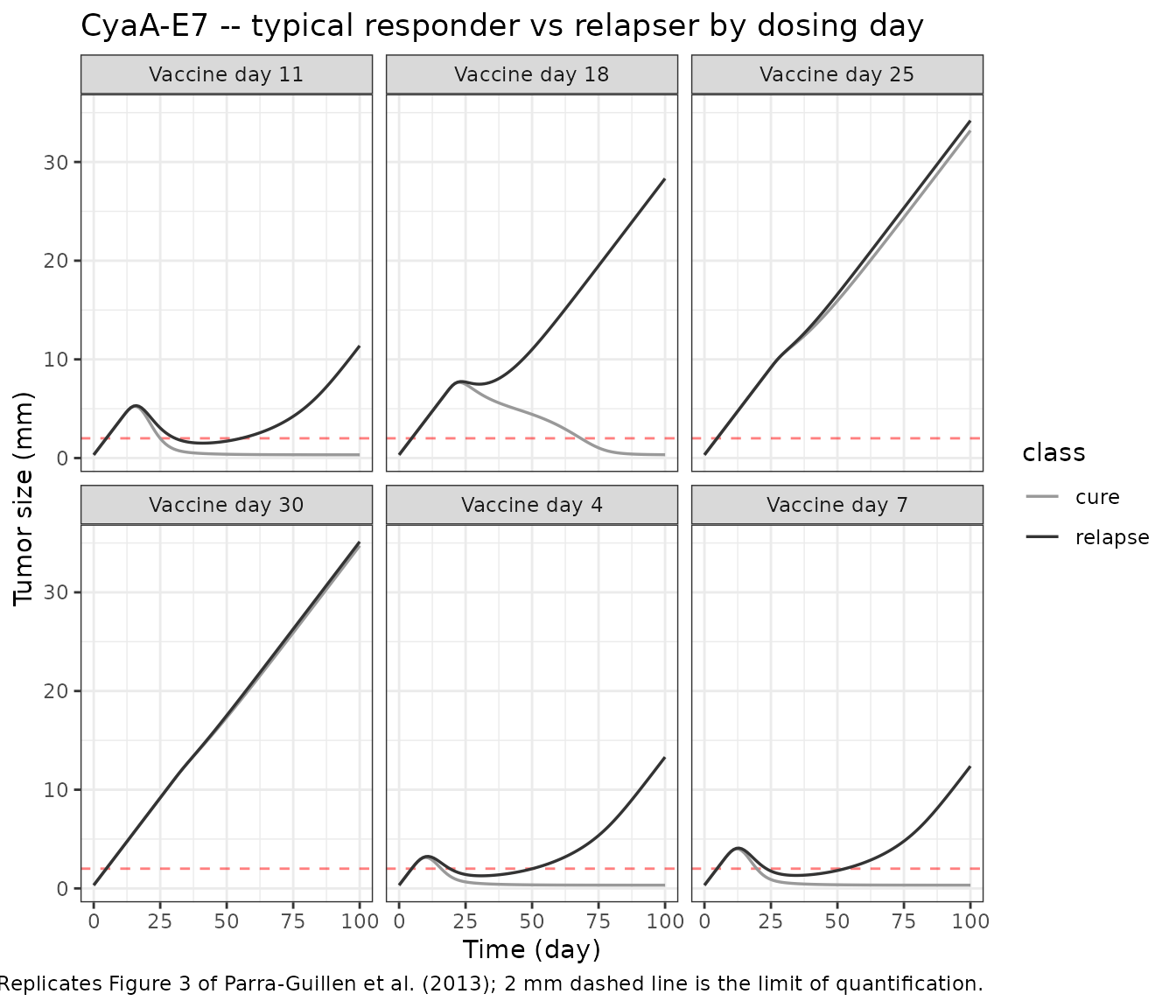
Vaccine administration at day 4, 7, or 11 (left column) produces a sharp drop in tumor size with the cure subpopulation reaching BQL and the relapser bouncing back. At day 18 and beyond the regulator compartment has accumulated enough to attenuate the vaccine-efficacy term (Eq. 4), so the cure trajectory is shallower and the relapser barely deflects – the source narrative describes this as “tumour size profiles were very similar to those obtained from the control group” at day 30 (Results, page 799).
CyaA-E7: VPC-style population predictions
For Figure 4, the source authors simulated 1000 datasets matching the study design and plotted the 50th percentile with 90% prediction interval. We reproduce the same VPC envelope at one dosing day with a smaller (but still informative) simulation, with the mixture-class assignment drawn Bernoulli per mouse.
sim_one_day <- function(model, dose_day, n = 200, tmax = 100,
                        p_relapse = 1 - 0.844, id_offset = 0L) {
  set.seed(dose_day + id_offset)
  mix <- as.integer(stats::runif(n) < p_relapse)
  ev  <- make_cohort(n = n, dose_day = dose_day, mix_relapse = mix,
                     tmax = tmax, id_offset = id_offset)
  out <- as.data.frame(rxode2::rxSolve(model, ev, nSub = 1L,
                                       keep = "MIX_VAC_RELAPSE"))
  out$dose_day <- dose_day
  out
}

cyaa_vpc_days <- c(4, 11, 18, 25)
cyaa_vpc <- bind_rows(lapply(seq_along(cyaa_vpc_days), function(i) {
  sim_one_day(mod_cyaa, dose_day = cyaa_vpc_days[i],
              n = 200, id_offset = i * 1000L)
}))
#> ℹ parameter labels from comments will be replaced by 'label()'
#> ℹ parameter labels from comments will be replaced by 'label()'
#> ℹ parameter labels from comments will be replaced by 'label()'
#> ℹ parameter labels from comments will be replaced by 'label()'

cyaa_vpc_summary <- cyaa_vpc |>
  group_by(dose_day, time) |>
  summarise(
    q05 = quantile(tumor_size, 0.05, na.rm = TRUE),
    q50 = quantile(tumor_size, 0.50, na.rm = TRUE),
    q95 = quantile(tumor_size, 0.95, na.rm = TRUE),
    .groups = "drop"
  )

ggplot(cyaa_vpc_summary, aes(time, q50)) +
  geom_hline(yintercept = 2, linetype = "dashed", colour = "red", alpha = 0.5) +
  geom_ribbon(aes(ymin = q05, ymax = q95), fill = "grey80", alpha = 0.6) +
  geom_line(linewidth = 0.7) +
  geom_vline(aes(xintercept = dose_day), linetype = "dotted",
             colour = "goldenrod") +
  facet_wrap(~ paste0("Vaccine day ", dose_day)) +
  labs(x = "Time (day)", y = "Tumor size (mm)",
       title = "CyaA-E7 -- simulated VPC by dosing day",
       caption = paste0(
         "Replicates Figure 4 of Parra-Guillen et al. (2013); ribbon = ",
         "5-95th percentile, line = median; gold dotted line = vaccine day.")) +
  theme_bw()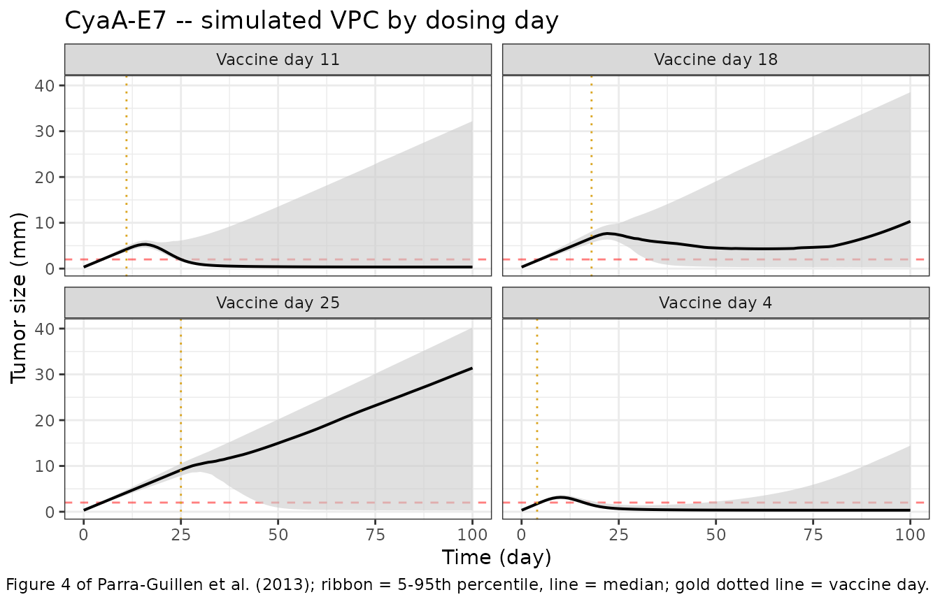
The widening percentile envelope across vaccine-administration arms reflects the empirical mixture: at day 4 most mice are cured (median collapses to BQL within ~20 days); at day 25 the regulator-driven resistance limits the vaccine effect (median tracks the control trajectory).
CyaA-E7: probability of cure by dosing day
Figure 5 of the source plots the simulated probability of cure (percent of mice with predicted Ts <= 2 mm at the end of the experiment) for each dosing group. We reproduce that summary with a larger simulation per arm.
end_of_study <- 60   # day used by the source for the "end-of-study" cure metric
cyaa_cure <- bind_rows(lapply(seq_along(cyaa_days), function(i) {
  sim_one_day(mod_cyaa, dose_day = cyaa_days[i], n = 200, tmax = end_of_study,
              id_offset = 10000L + i * 1000L)
})) |>
  filter(time == end_of_study) |>
  group_by(dose_day) |>
  summarise(prob_cure = mean(tumor_size <= 2, na.rm = TRUE), .groups = "drop")
#> ℹ parameter labels from comments will be replaced by 'label()'
#> ℹ parameter labels from comments will be replaced by 'label()'
#> ℹ parameter labels from comments will be replaced by 'label()'
#> ℹ parameter labels from comments will be replaced by 'label()'
#> ℹ parameter labels from comments will be replaced by 'label()'
#> ℹ parameter labels from comments will be replaced by 'label()'

cyaa_cure |>
  dplyr::rename(
    "Vaccine dose day"  = dose_day,
    "Simulated P(cure)" = prob_cure
  ) |>
  knitr::kable(
    caption = paste0("Simulated probability of cure at end of study (",
end_of_study, " days) -- CyaA-E7."))| Vaccine dose day | Simulated P(cure) |
|---|---|
| 4 | 0.835 |
| 7 | 0.805 |
| 11 | 0.720 |
| 18 | 0.485 |
| 25 | 0.125 |
| 30 | 0.050 |
ggplot(cyaa_cure, aes(dose_day, prob_cure)) +
  geom_col(width = 1.2, fill = "grey60") +
  scale_y_continuous(limits = c(0, 1)) +
  labs(x = "Vaccine dose day",
       y = "Simulated probability of cure",
       title = "CyaA-E7 -- probability of cure by dosing day",
       caption = paste0("Replicates Figure 5 of Parra-Guillen et al. ",
                        "(2013); probability of cure = fraction with ",
                        "tumor_size <= 2 mm at the end of study.")) +
  theme_bw()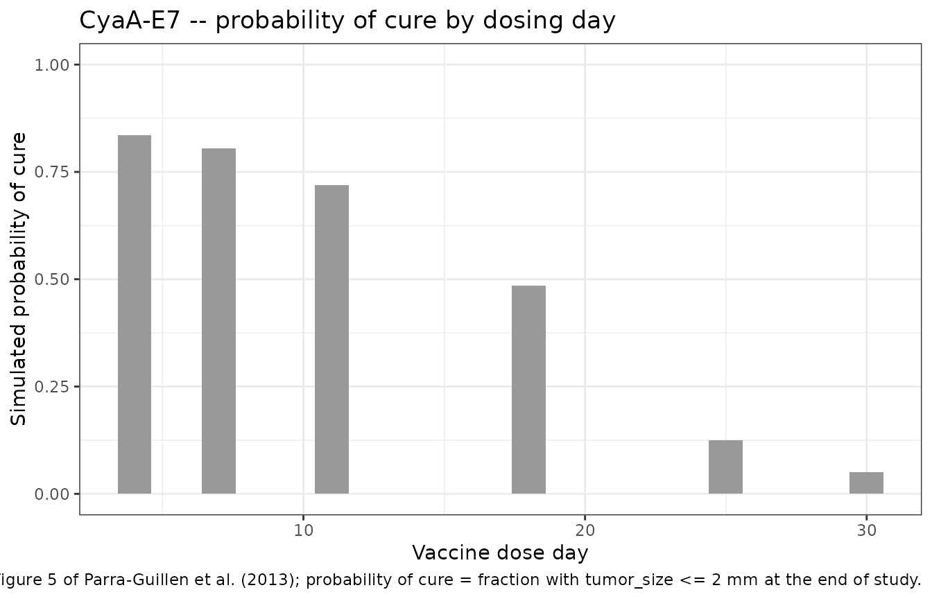
The simulated cure rate is at or near the responder ceiling of ~84 %
(the fixed mixture probability P(1)) for early vaccine
administration days, declining as resistance builds for later doses –
the dominant mechanism captured by the model.
IL-12 applicability: typical and population predictions
The IL-12 cohort received a single hydrodynamic plasmid injection on day 23. The simulation below shows the typical responder vs relapser trajectories and the VPC envelope; both reproduce the qualitative pattern in Figure 4 lower-right panel of the source.
mod_il12     <- readModelDb("ParraGuillen_2013_il12")
#> ℹ IL-12 plasmid dose enters the vac compartment as a unit bolus (amt = 1, cmt = vac). MIX_VAC_RELAPSE (0 = cure / responder, 1 = relapser; population probability of 1 is 1 - P(1) = 0.156, fixed from CyaA-E7) must be supplied per subject. Parameters k3 / k4 / gamma / P(1) are FIXED at the CyaA-E7 fit values; only Ts0 / lambda / k1 / REG50 (+ IAV) are re-estimated for the Medina-Echeverz MC38 cohort.
mod_il12_typ <- rxode2::zeroRe(mod_il12)
#> ℹ parameter labels from comments will be replaced by 'label()'

# Typical individuals
il12_typ <- bind_rows(lapply(c(0L, 1L), function(m) {
  ev <- make_cohort(n = 1, dose_day = 23, mix_relapse = m, tmax = 60,
                    id_offset = m + 1L)
  s <- as.data.frame(rxode2::rxSolve(mod_il12_typ, ev,
                                     keep = "MIX_VAC_RELAPSE"))
  s$class <- ifelse(m == 1L, "relapse", "cure")
  s
}))
#> ℹ omega/sigma items treated as zero: 'etallam', 'etalreg50'
#> ℹ omega/sigma items treated as zero: 'etallam', 'etalreg50'

# Population VPC
il12_vpc <- sim_one_day(mod_il12, dose_day = 23, n = 200, tmax = 60,
                       id_offset = 20000L)
#> ℹ parameter labels from comments will be replaced by 'label()'
il12_vpc_sum <- il12_vpc |>
  group_by(time) |>
  summarise(
    q05 = quantile(tumor_size, 0.05, na.rm = TRUE),
    q50 = quantile(tumor_size, 0.50, na.rm = TRUE),
    q95 = quantile(tumor_size, 0.95, na.rm = TRUE),
    .groups = "drop"
  )

ggplot(il12_vpc_sum, aes(time, q50)) +
  geom_hline(yintercept = 2, linetype = "dashed", colour = "red", alpha = 0.5) +
  geom_ribbon(aes(ymin = q05, ymax = q95), fill = "grey80", alpha = 0.6) +
  geom_line(linewidth = 0.7) +
  geom_line(data = il12_typ, aes(time, tumor_size, colour = class, group = class),
            inherit.aes = FALSE, linewidth = 0.8) +
  geom_vline(xintercept = 23, linetype = "dotted", colour = "goldenrod") +
  scale_colour_manual(values = c("cure" = "steelblue", "relapse" = "firebrick")) +
  labs(x = "Time (day)", y = "Tumor size (mm)",
       title = "IL-12 day 23 -- typical (lines) + VPC (ribbon)",
       caption = paste0("Replicates Figure 4 lower-right of Parra-Guillen ",
                        "et al. (2013); gold dotted line = IL-12 day.")) +
  theme_bw()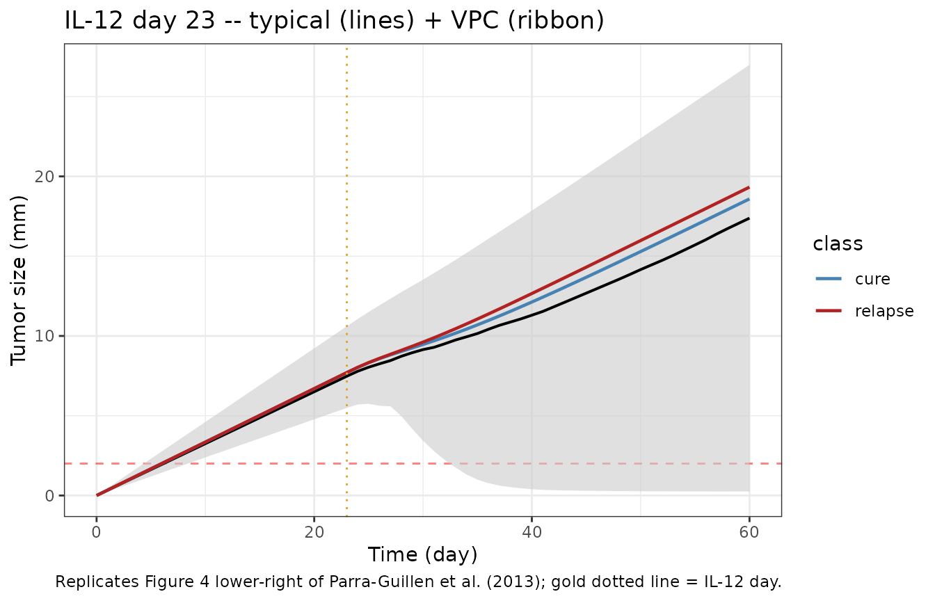
IL-12: probability of cure
il12_cure <- il12_vpc |>
  filter(time == 60) |>
  summarise(prob_cure = mean(tumor_size <= 2, na.rm = TRUE))
il12_cure |>
  dplyr::rename("Simulated P(cure) at day 60" = prob_cure) |>
  knitr::kable(
caption = "IL-12 day 23 simulated probability of cure at day 60.")| Simulated P(cure) at day 60 |
|---|
| 0.145 |
The simulated cure rate sits close to the responder ceiling (84 %), as expected for a vaccine-administration scheme that precedes substantial resistance accumulation under the cell-line-specific REG50 = 2.08 mm.
Assumptions and deviations
-
Mixture-class assignment.
MIX_VAC_RELAPSEis supplied per subject in the simulation event table. Typical-value figures (Figure 3 reproductions) setmix_relapseto a fixed 0 or 1. Population figures (Figure 4 / 5 reproductions) drawmix_relapse ~ Bernoulli(0.156)per mouse, matching the fixed mixture probabilityP(1) = 0.844reported by the paper. -
BQL handling at the simulation stage. The model
itself does not impose the 2 mm BQL censoring; simulated
tumor_sizevalues can go below 2 mm and even slightly negative under extreme parameter combinations. The probability-of-cure calculation thresholds attumor_size <= 2 mmto mirror the paper’s definition (Methods ‘Visual predictive checks’ / ‘Numerical Predictive Checks’ subsections, p. 800). -
Residual error encoding. The paper reports an
additive residual on log-transformed tumor diameter (Methods ‘Model
Building and Selection’, p. 798); the model file encodes this as
tumor_size ~ lnorm(expSd). The two forms are mathematically equivalent (additive onlog(Ts)<=> log-normal onTs). -
Cohort sizes in the vignette. The source authors
simulated 1000 populations per study design (Methods ‘Model Evaluation
and Validation’, p. 800); the vignette uses 200 per arm to keep the
render time within the pkgdown CI budget (5 minutes). The qualitative
shape of the VPC envelope is preserved; tighter percentile bands can be
obtained by raising
nin thesim_one_day()calls above. - Validation dataset. The 34-mouse external-validation cohort (PBS day 4, CyaA-E7 day 25) is described in the source but is not separately reproduced here because it shares the structural model with the training arms; the vaccine-day-25 panel in the CyaA-E7 VPC figure exercises the same conditions.
-
External datasets. The original observed data are
not redistributed with
nlmixr2lib; the figures above use simulated cohorts only. The Berraondo 2007 (CyaA-E7) and Medina-Echeverz 2014 (IL-12) experimental data remain in the original publications.