Carprofen tissue-cage PK with moxidectin as an internal standard (Munn 2024) • nlmixr2lib

mod_raw <- rxode2::rxode(readModelDb("Munn_2024_carprofen_raw"))
#> ℹ parameter labels from comments will be replaced by 'label()'
mod_cor <- rxode2::rxode(readModelDb("Munn_2024_carprofen_moxidectinCorrected"))
#> ℹ parameter labels from comments will be replaced by 'label()'

Model and source

Citation: Munn R, Whittem T. Moxidectin is a candidate for use as an in vivo internal standard in pharmacokinetic studies, as demonstrated with use in simultaneous tissue cage and ultrafiltration fluid collection. Front Vet Sci. 2024;11:1332974. doi:10.3389/fvets.2024.1332974. Parameter values from Supplementary Table S1, ‘Raw Analysis’ panel. The tissue-cage model structure is inherited from Munn R, Whittem T, Woodward AP. The surface area to volume ratio changes the pharmacokinetic and pharmacodynamic parameters in the subcutaneous tissue cage model: as illustrated by carprofen in sheep. Front Vet Sci. 2022;9:905797. doi:10.3389/fvets.2022.905797.
Article: https://doi.org/10.3389/fvets.2024.1332974
Supplement (Supplementary Table S1, the only place the parameter estimates appear): https://www.frontiersin.org/articles/10.3389/fvets.2024.1332974/full#supplementary-material
Upstream structural model: Munn, Whittem & Woodward (2022), https://doi.org/10.3389/fvets.2022.905797

This paper is primarily a methods paper: it asks whether moxidectin, given subcutaneously two weeks ahead and held at a pseudo-steady state by its ~18 day half-life, can serve as an in vivo internal standard that corrects for variable analyte recovery from tissue-fluid sampling. Carprofen is the probe drug. The authors fit their tissue-cage PK model twice – once to the raw carprofen concentrations and once to concentrations corrected by the concurrent moxidectin result – and compared the two. Both fits are packaged here:

nlmixr2lib::modeldb |>
  dplyr::filter(grepl("^Munn_2024", name)) |>
  dplyr::mutate(Description = paste0(substr(description, 1, 90), "...")) |>
  dplyr::select(Model = name, Description) |>
  knitr::kable()

Model	Description
Munn_2024_carprofen_moxidectinCorrected	Preclinical (sheep). Three-compartment population PK model for carprofen after a single 4 …
Munn_2024_carprofen_raw	Preclinical (sheep). Three-compartment population PK model for carprofen after a single 4 …

Where the parameter values come from

The main text deliberately withholds the estimates: “The precise estimates are available in the Supplementary Table S1, but are not reported, as discussed below.” The Discussion explains why – the authors regard this dataset’s estimates as internally comparable but less externally valid than their 2022 study, because only two cage sizes were used and large analytical corrections were needed. Every number in the two model files is therefore taken from Supplementary Table S1, not from the article body. Figure 1 of the article plots the same estimates with confidence intervals but does not print them.

The structure of the model is not described in this paper either – Methods 2.2 says only that the fit used “a custom model as previously described (16)”. Reference 16 is Munn, Whittem & Woodward (2022), and the structural description below is taken from that paper’s Results / Figure 1.

Population

Eight merino wethers (castrated male sheep), approximately 18 months old, weighing 42-51.5 kg, judged healthy on clinical examination plus routine haematology and biochemistry. Two subcutaneous tissue cages (6 cm and 10 cm length) were implanted in the neck three weeks before the study, so every animal contributes both cage sizes simultaneously. Moxidectin 0.2 mg/kg was injected subcutaneously into a hind limb 14 days before the experiment; at time zero carprofen 4 mg/kg was given as an intravenous bolus into a cephalic vein. Plasma and tissue-cage fluid were sampled at -0.5, 0.5, 1, 2, 3, 4, 5, 7, 24, 36, 48 and 72 h.

Ultrafiltration probes were inserted on the morning of the study as well, but they failed to yield enough sample volume: of 74 ultrafiltrate samples, carprofen was quantifiable in 71 and moxidectin in only 19, and 66 of the carprofen results were below 1 ng/mL. Results 3.1 states plainly that “insufficient valid results were available from the ultrafiltration probes to perform analysis on these data”. There is therefore no ultrafiltration compartment in the model, and none appears in these files.

str(mod_raw$population)
#> List of 10
#>  $ species       : chr "sheep (merino wether)"
#>  $ n_subjects    : int 8
#>  $ n_studies     : int 1
#>  $ age_range     : chr "approximately 18 months"
#>  $ weight_range  : chr "42-51.5 kg"
#>  $ sex_female_pct: num 0
#>  $ disease_state : chr "Healthy (veterinary clinical examination plus routine haematology and biochemistry before enrolment)"
#>  $ dose_range    : chr "Single 4 mg/kg carprofen intravenous bolus into a cephalic vein at time zero. Separately, 0.2 mg/kg moxidectin "| __truncated__
#>  $ regions       : chr "Australia (University of Melbourne, Werribee, Victoria)"
#>  $ notes         : chr "Two tissue cages (6 cm and 10 cm length) were implanted subcutaneously in the neck three weeks before the exper"| __truncated__

Model structure

Taken from Munn 2022 (Results, “Pharmacokinetic Model”, and its Figure 1):

Plasma disposition is a two-compartment model, built first and fitted to the intravenous plasma data alone, parameterised in Monolix micro-constant form as central volume Vc, clearance CL, and rate constants k12 / k21.
A tissue-cage compartment was then appended. Its concentration is driven by the central-compartment concentration through a first-order rate k13 in and k31 out, and – crucially – it does not feed back into the central compartment: “The rates of influx and efflux are first order and are driven by the central compartment concentrations without altering the central compartment concentrations.” Only a negligible fraction of the dose enters a cage, so this is the classical negligible-mass (Sheiner-style) construction.
Cage size modifies k13 and k31.

Because each sheep carried a 6 cm and a 10 cm cage at the same time, the model files carry two cage states, cage6 and cage10, solved simultaneously and each driven by the same plasma profile. Both hold a concentration (ug/mL) rather than an amount, which is what a state driven by Cc with no mass transfer represents.

cat(paste(vapply(mod_raw$lstExpr, deparse1, character(1)), collapse = "\n"))
#> vc <- exp(lvc + etalvc)
#> cl <- exp(lcl + etalcl)
#> k12 <- exp(lk12 + etalk12)
#> k21 <- exp(lk21 + etalk21)
#> k13_cage6 <- exp(lk13)
#> k31_cage6 <- exp(lk31)
#> k13_cage10 <- exp(lk13 + e_cage10_k13)
#> k31_cage10 <- exp(lk31 + e_cage10_k31)
#> kel <- cl/vc
#> d/dt(central) <- k21 * peripheral1 - k12 * central - kel * central
#> d/dt(peripheral1) <- k12 * central - k21 * peripheral1
#> Cc <- central/vc
#> d/dt(cage6) <- k13_cage6 * Cc - k31_cage6 * cage6
#> d/dt(cage10) <- k13_cage10 * Cc - k31_cage10 * cage10
#> Ccage6 <- cage6
#> Ccage10 <- cage10
#> Cc ~ prop(propSd)
#> Ccage6 ~ prop(propSd_Ccage6)
#> Ccage10 ~ prop(propSd_Ccage10)

Source trace

Every value below is from Supplementary Table S1 of Munn 2024 unless noted. The Raw column is the “Raw Analysis” panel; the Corrected column is the “Moxidectin Corrected” panel. Relative standard errors are the table’s own R.S.E.(%) column.

Parameter	Model name	Raw	Corrected	Source
Central volume (L/kg)	`lvc`	0.045 (RSE 4.69%)	0.045 (RSE 4.80%)	Suppl Table S1, Fixed Effects
Clearance (L/h/kg)	`lcl`	0.0016 (RSE 5.54%)	0.0016 (RSE 5.52%)	Suppl Table S1, Fixed Effects
k12 (1/h)	`lk12`	0.11 (RSE 40.7%)	0.12 (RSE 40.9%)	Suppl Table S1, Fixed Effects
k21 (1/h)	`lk21`	0.30 (RSE 32.2%)	0.32 (RSE 31.8%)	Suppl Table S1, Fixed Effects
k13, 6 cm cage (1/h)	`lk13`	0.052 (RSE 25.3%)	0.053 (RSE 25.3%)	Suppl Table S1, Fixed Effects
k31, 6 cm cage (1/h)	`lk31`	0.22 (RSE 35.8%)	0.21 (RSE 35.9%)	Suppl Table S1, Fixed Effects
k13 effect, 10 cm vs 6 cm	`e_cage10_k13`	-0.056 (RSE 54.0%)	-0.057 (RSE 53.1%)	Suppl Table S1; 6 cm row printed as `0*`
k31 effect, 10 cm vs 6 cm	`e_cage10_k31`	-0.17 (RSE 26.5%)	-0.17 (RSE 27.0%)	Suppl Table S1; 6 cm row printed as `0*`
IIV Vc (log-scale SD)	`etalvc`	0.000091	0.00026	Suppl Table S1, SD of Random Effects
IIV k12 (log-scale SD)	`etalk12`	0.42	0.41	Suppl Table S1, SD of Random Effects
IIV k21 (log-scale SD)	`etalk21`	0.00052	0.00089	Suppl Table S1, SD of Random Effects
IIV CL (log-scale SD)	`etalcl`	0.13	0.13	Suppl Table S1, SD of Random Effects
Residual error	`propSd*`	not reported	not reported	absent from Suppl Table S1; fixed to 0
Structural form	`model()`	–	–	Munn 2022 Results + Figure 1

The scale of the cage-size coefficients

Supplementary Table S1 labels the cage-size rows with the unit (h-1), which would suggest an additive effect on the rate constant. That reading is wrong, and the paper’s own numbers falsify it: k13 for the 10 cm cage would be 0.052 + (-0.056) = -0.004 per hour, a negative rate constant.

The coefficients are Monolix’s default for a log-normally distributed parameter, i.e. multiplicative on the natural scale: k_10cm = k_6cm * exp(beta). A second, independent confirmation comes from the upstream paper. Munn 2022 fitted the same covariate as a continuous per-cm effect (k31 -0.147 and k13 -0.0378 on k31 = 0.455, k13 = 0.124) and tabulated the resulting median rate constants by cage size in its Table 5. The log-scale reading reproduces that table across the whole 0-18 cm range, while the additive reading goes negative from 4 cm onward:

cage_cm <- c(0, 3, 6, 10, 14, 18)
tibble::tibble(
  `Cage size (cm)`            = cage_cm,
  `k13 log-scale`             = round(0.124 * exp(-0.0378 * cage_cm), 4),
  `k13 Munn 2022 Table 5`     = c(0.1390, 0.1060, 0.1140, 0.0862, 0.0582, 0.0694),
  `k13 additive`              = round(0.124 - 0.0378 * cage_cm, 4),
  `k31 log-scale`             = round(0.455 * exp(-0.147 * cage_cm), 4),
  `k31 Munn 2022 Table 5`     = c(0.5190, 0.3860, 0.1530, 0.0703, 0.0513, 0.0400),
  `k31 additive`              = round(0.455 - 0.147 * cage_cm, 4)
) |>
  knitr::kable(caption = "Log-scale vs additive readings against Munn 2022 Table 5 median rate constants.")

Log-scale vs additive readings against Munn 2022 Table 5 median rate constants.
Cage size (cm)	k13 log-scale	k13 Munn 2022 Table 5	k13 additive	k31 log-scale	k31 Munn 2022 Table 5	k31 additive
0	0.1240	0.1390	0.1240	0.4550	0.5190	0.455
3	0.1107	0.1060	0.0106	0.2927	0.3860	0.014
6	0.0988	0.1140	-0.1028	0.1883	0.1530	-0.427
10	0.0850	0.0862	-0.2540	0.1046	0.0703	-1.015
14	0.0730	0.0582	-0.4052	0.0581	0.0513	-1.603
18	0.0628	0.0694	-0.5564	0.0323	0.0400	-2.191


# The additive reading is not merely less accurate -- it is impossible.
stopifnot(
  any(0.124 - 0.0378 * cage_cm < 0),
  any(0.455 - 0.147 * cage_cm < 0),
  all(0.124 * exp(-0.0378 * cage_cm) > 0),
  all(0.455 * exp(-0.147 * cage_cm) > 0)
)

Categorical, not continuous

Methods 2.2 of Munn 2024 says cage length “in centimeters” was “used as the regressor value” and calls it “a continuous co-variate”. Supplementary Table S1 contradicts that: it prints a reference row Covariate for k13 for Cage Size 6 cm = 0* and a single estimated offset for the 10 cm cage. 0* is Monolix’s fixed-reference marker for a categorical covariate. The same authors’ 2022 table distinguishes the two forms explicitly, printing continuous effects as “Covariate for k31 per cm Cage size” and categorical ones with a 0* reference row – and the 2024 table uses the categorical form. With only two cage sizes in this study the two parameterisations are equivalent in fit, and the prose appears to be carried over from the 2022 methods. The model files follow the table.

Simulation

The source reports Vc in L/kg and CL in L/h/kg, and doses in mg/kg, so the models are coded on a per-kilogram basis: the dosed amount is mg/kg, the volume is L/kg, and central / vc lands directly in mg/L, which is ug/mL – the units of the carprofen assay (calibration range 0.25-100 ug/mL, Methods 2.1).

DOSE_MGKG <- 4      # Munn 2024 Methods: 4 mg/kg carprofen IV bolus at time zero
T_END     <- 72     # the paper's sampling window

make_events <- function(n_sub, t_end = T_END, by = 0.25) {
  obs <- tidyr::expand_grid(
    id   = seq_len(n_sub),
    time = sort(unique(c(seq(0, t_end, by = by), c(0.5, 1, 2, 3, 4, 5, 7, 24, 36, 48, 72))))
  ) |>
    dplyr::mutate(amt = NA_real_, evid = 0L, cmt = "central", dvid = 1L)
  dose <- tibble::tibble(
    id = seq_len(n_sub), time = 0, amt = DOSE_MGKG, evid = 1L,
    cmt = "central", dvid = NA_integer_
  )
  dplyr::bind_rows(dose, obs) |>
    dplyr::arrange(id, time, dplyr::desc(evid)) |>
    as.data.frame()
}

Observation rows are tagged with the ODE state central and dvid = 1; the models declare three endpoints (Cc, Ccage6, Ccage10), so the dvid tag is what resolves the endpoint mapping. Every algebraic observable is still returned on every solved row. useLinCmt = FALSE avoids rxode2’s automatic ODE-to-linCmt() conversion, which corrupts the dvid mapping for multi-output models of this shape.

ev1 <- make_events(1)

solve_typical <- function(mod) {
  rxode2::rxSolve(mod, ev1, omega = NA, returnType = "data.frame",
                  addDosing = FALSE, useLinCmt = FALSE)
}
tv_raw <- solve_typical(mod_raw)
tv_cor <- solve_typical(mod_cor)

Typical-value profiles

prof <- dplyr::bind_rows(
  dplyr::mutate(tv_raw, Fit = "Raw"),
  dplyr::mutate(tv_cor, Fit = "Moxidectin-corrected")
) |>
  dplyr::select(Fit, time, Plasma = Cc, `Cage 6 cm` = Ccage6, `Cage 10 cm` = Ccage10) |>
  tidyr::pivot_longer(c(Plasma, `Cage 6 cm`, `Cage 10 cm`),
                      names_to = "Matrix", values_to = "conc") |>
  dplyr::mutate(Matrix = factor(Matrix, levels = c("Plasma", "Cage 6 cm", "Cage 10 cm")))

ggplot(prof, aes(time, conc, colour = Matrix, linetype = Fit)) +
  geom_line(linewidth = 0.7) +
  scale_y_log10() +
  scale_x_continuous(breaks = seq(0, 72, 12)) +
  labs(x = "Time (h)", y = "Carprofen (ug/mL)",
       colour = NULL, linetype = NULL) +
  theme_bw() +
  theme(legend.position = "bottom")
#> Warning in scale_y_log10(): log-10 transformation introduced infinite values.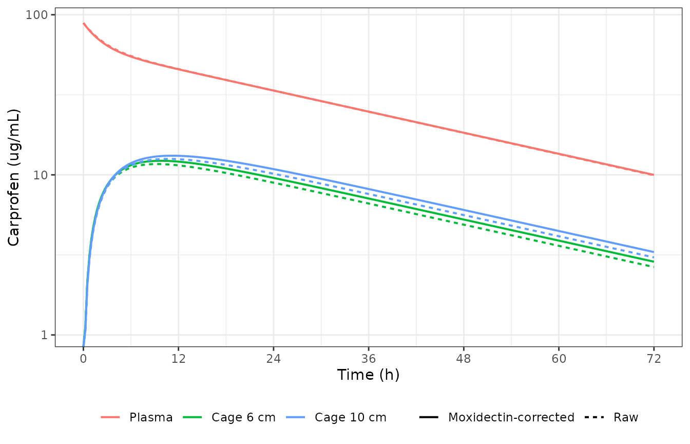

Typical-value carprofen concentrations in plasma and in the two tissue cages after a single 4 mg/kg IV bolus, for the raw and moxidectin-corrected fits.

The two fits are visually indistinguishable, which is the paper’s central finding.

Validation

Closed-form identities

The typical-value solve is deterministic, so these are exact algebraic identities rather than statistical comparisons, and are asserted tightly.

theta <- function(ui, nm) {
  v <- ui$iniDf$est[ui$iniDf$name == nm]
  stopifnot(length(v) == 1L)
  v
}
vc_raw <- exp(theta(mod_raw, "lvc"))
cl_raw <- exp(theta(mod_raw, "lcl"))

# C0 = Dose / Vc
c0_pred <- tv_raw$Cc[tv_raw$time == 0]
c0_theo <- DOSE_MGKG / vc_raw
stopifnot(length(c0_pred) == 1L, abs(c0_pred / c0_theo - 1) < 1e-8)

# Cage plateau ratio -> k13 / k31 (each cage independently)
k13_6  <- exp(theta(mod_raw, "lk13"))
k31_6  <- exp(theta(mod_raw, "lk31"))
k13_10 <- exp(theta(mod_raw, "lk13") + theta(mod_raw, "e_cage10_k13"))
k31_10 <- exp(theta(mod_raw, "lk31") + theta(mod_raw, "e_cage10_k31"))

tibble::tibble(
  Check = c("C0 = Dose/Vc (ug/mL)",
            "Cage 6 cm equilibrium ratio k13/k31",
            "Cage 10 cm equilibrium ratio k13/k31"),
  Model = c(round(c0_pred, 4), round(k13_6 / k31_6, 4), round(k13_10 / k31_10, 4)),
  `Closed form` = c(round(c0_theo, 4), round(k13_6 / k31_6, 4), round(k13_10 / k31_10, 4))
) |>
  knitr::kable(caption = "Deterministic identities from the typical-value solve.")

Deterministic identities from the typical-value solve.
Check	Model	Closed form
C0 = Dose/Vc (ug/mL)	88.8889	88.8889
Cage 6 cm equilibrium ratio k13/k31	0.2364	0.2364
Cage 10 cm equilibrium ratio k13/k31	0.2649	0.2649

The published half-life

This is the one numeric result the article body does print, and it is a genuine external check on the transcription of Vc and CL. The Discussion states: “This resulted in an estimated half-life of 19.5 h compared to 27.2 h in the previous dataset.” Both numbers are reproduced exactly as ln(2) / (CL / Vc) – the central-compartment half-life:

t_half_central <- function(cl, vc) log(2) / (cl / vc)

halflife <- tibble::tibble(
  Study      = c("Munn 2024 (this paper)", "Munn 2022 (previous dataset)"),
  `Vc (L/kg)`   = c(0.045, 0.0924),
  `CL (L/h/kg)` = c(0.0016, 0.00235),
  Computed   = t_half_central(c(0.0016, 0.00235), c(0.045, 0.0924)),
  Published  = c(19.5, 27.2)
) |>
  dplyr::mutate(Computed = round(Computed, 2))
knitr::kable(halflife, caption = "ln(2)/(CL/Vc) against the half-lives printed in Munn 2024 Discussion.")

ln(2)/(CL/Vc) against the half-lives printed in Munn 2024 Discussion.
Study	Vc (L/kg)	CL (L/h/kg)	Computed	Published
Munn 2024 (this paper)	0.0450	0.00160	19.49	19.5
Munn 2022 (previous dataset)	0.0924	0.00235	27.25	27.2


# Tolerance 0.15 h reflects the 2-3 significant figures the source prints for
# Vc and CL; it is not slack. Perturbing either input by one unit in its last
# printed digit (Vc 0.045 -> 0.046, CL 0.0016 -> 0.0017) moves the computed
# half-life by 0.4-1.2 h, so a single mis-transcribed digit fails this check.
stopifnot(all(abs(halflife$Computed - halflife$Published) < 0.15))

Because a single printed number pins the ratio CL / Vc for both studies, and Vc is separately pinned by C0 = Dose / Vc, this confirms both transcribed values rather than just their ratio.

Note that 19.5 h is not the terminal half-life of the two-compartment system, which for this parameter set is longer:

terminal_half <- function(k12, k21, kel) {
  b    <- k12 + k21 + kel
  beta <- (b - sqrt(b^2 - 4 * k21 * kel)) / 2
  log(2) / beta
}
th <- terminal_half(exp(theta(mod_raw, "lk12")), exp(theta(mod_raw, "lk21")),
                    cl_raw / vc_raw)
cat(sprintf("Terminal half-life of the raw fit: %.1f h\n", th))
#> Terminal half-life of the raw fit: 27.3 h

NCA on the simulated plasma profile

Non-compartmental analysis of the typical-value plasma profile must return AUC(0-inf) = Dose / CL. The NCA uses a grid extended well beyond the paper’s 72 h sampling window so that the terminal slope is well characterised and the extrapolated fraction is small; the 72 h window above is retained for the figures.

ev_nca <- make_events(1, t_end = 336, by = 0.25)
nca_sim <- rxode2::rxSolve(mod_raw, ev_nca, omega = NA, returnType = "data.frame",
                           addDosing = FALSE, useLinCmt = FALSE)

conc_df <- nca_sim |>
  dplyr::transmute(id = 1L, time, Cc, treatment = "4 mg/kg IV") |>
  dplyr::filter(!is.na(Cc))
stopifnot(nrow(conc_df) > 0, any(conc_df$time == 0), all(conc_df$Cc >= 0))

dose_df <- tibble::tibble(id = 1L, time = 0, amount = DOSE_MGKG,
                          treatment = "4 mg/kg IV")

o_conc <- PKNCA::PKNCAconc(conc_df, Cc ~ time | treatment + id,
                           concu = "ug/mL", timeu = "h")
o_dose <- PKNCA::PKNCAdose(dose_df, amount ~ time | treatment + id,
                           doseu = "mg/kg")
# aucpext.obs is not a PKNCA default, and it is the check that makes the
# aucinf comparison meaningful (it bounds how much of the reported AUC is
# extrapolated past the last simulated point), so the intervals are named
# explicitly rather than left to the default set.
nca_intervals <- data.frame(
  start = 0, end = Inf,
  cmax = TRUE, tmax = TRUE, auclast = TRUE,
  aucinf.obs = TRUE, aucpext.obs = TRUE, half.life = TRUE
)
res    <- PKNCA::pk.nca(PKNCA::PKNCAdata(o_conc, o_dose,
                                         intervals = nca_intervals))

nca_tbl <- as.data.frame(res) |>
  dplyr::filter(PPTESTCD %in% c("cmax", "tmax", "aucinf.obs", "half.life",
                                "aucpext.obs")) |>
  dplyr::select(PPTESTCD, PPORRES)
knitr::kable(nca_tbl, caption = "PKNCA results for the typical-value plasma profile.")

PKNCA results for the typical-value plasma profile.
PPTESTCD	PPORRES
cmax	88.8888889
tmax	0.0000000
half.life	27.2496658
aucinf.obs	2500.0421524
aucpext.obs	0.0192004


get_nca <- function(code) {
  v <- nca_tbl$PPORRES[nca_tbl$PPTESTCD == code]
  if (length(v) != 1L) stop("no unique NCA row for ", code)
  v
}

auc_theo <- DOSE_MGKG / cl_raw
comparison <- tibble::tibble(
  `NCA parameter` = c("Cmax (ug/mL)", "AUC0-inf obs (ug*h/mL)",
                      "Terminal t1/2 (h)"),
  Simulated = round(c(get_nca("cmax"), get_nca("aucinf.obs"),
                      get_nca("half.life")), 3),
  `Closed form` = round(c(DOSE_MGKG / vc_raw, auc_theo, th), 3)
) |>
  dplyr::mutate(`Difference (%)` = round(100 * (Simulated / `Closed form` - 1), 3))
knitr::kable(comparison,
             caption = "Simulated NCA against the model's own closed-form values.")

Simulated NCA against the model’s own closed-form values.
NCA parameter	Simulated	Closed form	Difference (%)
Cmax (ug/mL)	88.889	88.889	0.000
AUC0-inf obs (ug*h/mL)	2500.042	2500.000	0.002
Terminal t1/2 (h)	27.250	27.304	-0.198


# Deterministic solve against its own algebra: numerical error only, so these
# are tight by design. A mis-transcribed dose, volume or clearance moves them
# by tens of percent.
stopifnot(
  abs(get_nca("aucinf.obs") / auc_theo - 1)          < 0.01,
  abs(get_nca("cmax") / (DOSE_MGKG / vc_raw) - 1)    < 1e-6,
  abs(get_nca("half.life") / th - 1)                 < 0.01,
  get_nca("aucpext.obs")                             < 5
)

NCA on the tissue cages

Each cage is a separate output, so it gets its own NCA pass. Unlike plasma, these profiles rise to a peak and there is no dose into the cage, so only the shape parameters are meaningful.

cage_nca <- function(col, label) {
  cdf <- nca_sim |>
    dplyr::transmute(id = 1L, time, conc = .data[[col]], treatment = label) |>
    dplyr::filter(!is.na(conc))
  stopifnot(nrow(cdf) > 0, any(cdf$time == 0), all(cdf$conc >= 0))
  oc <- PKNCA::PKNCAconc(cdf, conc ~ time | treatment + id,
                         concu = "ug/mL", timeu = "h")
  r  <- PKNCA::pk.nca(PKNCA::PKNCAdata(oc, intervals = data.frame(
    start = 0, end = 336, cmax = TRUE, tmax = TRUE, auclast = TRUE)))
  as.data.frame(r) |>
    dplyr::filter(PPTESTCD %in% c("cmax", "tmax", "auclast")) |>
    dplyr::transmute(Cage = label, PPTESTCD, PPORRES = round(PPORRES, 3))
}

cages <- dplyr::bind_rows(
  cage_nca("Ccage6",  "Cage 6 cm"),
  cage_nca("Ccage10", "Cage 10 cm")
) |>
  tidyr::pivot_wider(names_from = PPTESTCD, values_from = PPORRES) |>
  dplyr::rename("Cmax (ug/mL)" = cmax, "Tmax (h)" = tmax,
                "AUClast (ug*h/mL)" = auclast)
#> No dose information provided, calculations requiring dose will return NA.
#> No dose information provided, calculations requiring dose will return NA.
knitr::kable(cages, caption = "PKNCA shape parameters for the two tissue cages.")

PKNCA shape parameters for the two tissue cages.
Cage	AUClast (ug*h/mL)	Cmax (ug/mL)	Tmax (h)
Cage 6 cm	590.755	11.679	9.25
Cage 10 cm	662.091	12.572	10.75


tmax6  <- cages$`Tmax (h)`[cages$Cage == "Cage 6 cm"]
tmax10 <- cages$`Tmax (h)`[cages$Cage == "Cage 10 cm"]
# Both cages lag plasma (Tmax = 0 for an IV bolus) and the larger, slower cage
# peaks later -- the qualitative cage-size effect Munn 2022 reports. These are
# deterministic typical-value solves, so the ordering is not a coin flip.
stopifnot(tmax6 > 0, tmax10 > tmax6)

The larger cage peaks later, which is the direction Munn 2022 reports (its Table 4 gives median observed Tmax rising from 8 h for a 3 cm cage to 48 h for a 14 cm cage). Note that in this dataset the 10 cm cage also reaches a slightly higher peak than the 6 cm cage, whereas Munn 2022 found Cmax falling with cage size. That follows directly from the printed 2024 estimates – the equilibrium ratio k13/k31 is 0.236 for the 6 cm cage and 0.265 for the 10 cm cage – and is one concrete instance of the limited external validity the authors themselves flag.

Replicating Figure 1

Figure 1 of the article plots each estimated parameter for the raw (green) and moxidectin-corrected fits with 95% confidence intervals, to support the claim that “Correction of the carprofen concentrations using moxidectin concentrations did not alter the estimated values of the pharmacokinetic parameters. The degree of uncertainty for these values was unaffected as shown by the 95% confidence intervals.”

The figure itself prints no numbers, but Supplementary Table S1 gives the standard error of every estimate, so the intervals can be reconstructed as Wald intervals. The article generated its intervals with the Rsmlx package, which need not use the Wald approximation, so these are a reconstruction of the figure’s content rather than a pixel reproduction.

fig1 <- tibble::tribble(
  ~Parameter,                        ~Fit,                   ~Estimate, ~SE,
  "Central volume (L/kg)",           "Raw",                   0.045,    0.0021,
  "Central volume (L/kg)",           "Moxidectin-corrected",  0.045,    0.0021,
  "Clearance (L/h.kg)",              "Raw",                   0.0016,   0.000088,
  "Clearance (L/h.kg)",              "Moxidectin-corrected",  0.0016,   0.000087,
  "k12 (1/h)",                       "Raw",                   0.11,     0.044,
  "k12 (1/h)",                       "Moxidectin-corrected",  0.12,     0.048,
  "k21 (1/h)",                       "Raw",                   0.30,     0.096,
  "k21 (1/h)",                       "Moxidectin-corrected",  0.32,     0.100,
  "k13 (1/h)",                       "Raw",                   0.052,    0.013,
  "k13 (1/h)",                       "Moxidectin-corrected",  0.053,    0.013,
  "k31 (1/h)",                       "Raw",                   0.22,     0.078,
  "k31 (1/h)",                       "Moxidectin-corrected",  0.21,     0.076,
  "Covariate k13, 10 cm cage",       "Raw",                  -0.056,    0.030,
  "Covariate k13, 10 cm cage",       "Moxidectin-corrected", -0.057,    0.030,
  "Covariate k31, 10 cm cage",       "Raw",                  -0.17,     0.045,
  "Covariate k31, 10 cm cage",       "Moxidectin-corrected", -0.17,     0.045
) |>
  dplyr::mutate(lower = Estimate - 1.96 * SE, upper = Estimate + 1.96 * SE)

ggplot(fig1, aes(Estimate, Fit, colour = Fit)) +
  geom_point(size = 2) +
  geom_errorbarh(aes(xmin = lower, xmax = upper), height = 0.2) +
  facet_wrap(~Parameter, scales = "free_x", ncol = 2) +
  labs(x = "Estimate (95% CI)", y = NULL) +
  theme_bw() +
  theme(legend.position = "none")
#> Warning: `geom_errorbarh()` was deprecated in ggplot2 4.0.0.
#> ℹ Please use the `orientation` argument of `geom_errorbar()` instead.
#> This warning is displayed once per session.
#> Call `lifecycle::last_lifecycle_warnings()` to see where this warning was
#> generated.
#> `height` was translated to `width`.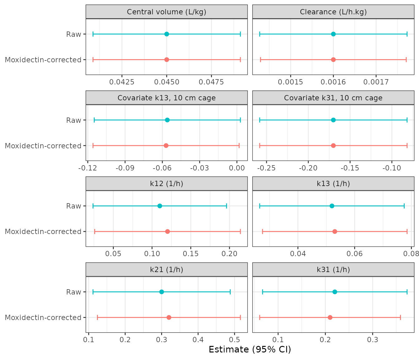

Replicates Figure 1 of Munn 2024: estimated parameters with 95% Wald confidence intervals, raw vs moxidectin-corrected.

Testing the paper’s headline claim

The claim has two halves: the estimates do not move, and the uncertainty does not change. Both are checkable from Supplementary Table S1.

claim <- fig1 |>
  tidyr::pivot_wider(id_cols = Parameter, names_from = Fit,
                     values_from = c(Estimate, SE, lower, upper)) |>
  dplyr::mutate(
    `Estimate shift (%)` = round(
      100 * (`Estimate_Moxidectin-corrected` - Estimate_Raw) /
        pmax(abs(Estimate_Raw), .Machine$double.eps), 2),
    `SE ratio` = round(`SE_Moxidectin-corrected` / SE_Raw, 3),
    `CIs overlap` = pmax(lower_Raw, `lower_Moxidectin-corrected`) <=
      pmin(upper_Raw, `upper_Moxidectin-corrected`)
  ) |>
  dplyr::select(Parameter, `Estimate shift (%)`, `SE ratio`, `CIs overlap`)
knitr::kable(claim, caption = "Raw vs moxidectin-corrected: shift in each estimate, ratio of standard errors, and whether the 95% CIs overlap.")

Raw vs moxidectin-corrected: shift in each estimate, ratio of standard errors, and whether the 95% CIs overlap.
Parameter	Estimate shift (%)	SE ratio	CIs overlap
Central volume (L/kg)	0.00	1.000	TRUE
Clearance (L/h.kg)	0.00	0.989	TRUE
k12 (1/h)	9.09	1.091	TRUE
k21 (1/h)	6.67	1.042	TRUE
k13 (1/h)	1.92	1.000	TRUE
k31 (1/h)	-4.55	0.974	TRUE
Covariate k13, 10 cm cage	-1.79	1.000	TRUE
Covariate k31, 10 cm cage	0.00	1.000	TRUE


stopifnot(
  # "did not alter the estimated values": every estimate moves by well under
  # its own standard error.
  all(abs(fig1$Estimate[fig1$Fit == "Moxidectin-corrected"] -
          fig1$Estimate[fig1$Fit == "Raw"]) < fig1$SE[fig1$Fit == "Raw"]),
  # "the degree of uncertainty ... was unaffected": SEs within 10% of each other.
  all(abs(claim$`SE ratio` - 1) < 0.10),
  # every interval overlaps its counterpart
  all(claim$`CIs overlap`)
)

Both halves of the claim hold on the paper’s own numbers: no estimate moves by as much as one standard error, no standard error changes by more than 10%, and every pair of confidence intervals overlaps.

Between-animal variability

A cohort simulation shows the spread the reported IIV produces. Only k12 and CL carry meaningful variability; the Vc and k21 random effects were driven to essentially zero by the estimator and are not identifiable (relative standard errors of 1.8e+7% and 2.7e+7% in the raw fit), so they are reproduced as reported but contribute nothing.

rxode2::rxSetSeed(20240116)
N_SHEEP <- 100                       # illustrative cohort; the study had 8
sim <- rxode2::rxSolve(mod_raw, make_events(N_SHEEP), returnType = "data.frame",
                       addDosing = FALSE, useLinCmt = FALSE)
if (is.null(sim$id)) sim$id <- 1L

sim |>
  dplyr::select(id, time, Plasma = Cc, `Cage 6 cm` = Ccage6, `Cage 10 cm` = Ccage10) |>
  tidyr::pivot_longer(c(Plasma, `Cage 6 cm`, `Cage 10 cm`),
                      names_to = "Matrix", values_to = "conc") |>
  dplyr::mutate(Matrix = factor(Matrix,
                                levels = c("Plasma", "Cage 6 cm", "Cage 10 cm"))) |>
  dplyr::group_by(Matrix, time) |>
  dplyr::summarise(med = median(conc),
                   lo  = quantile(conc, 0.05),
                   hi  = quantile(conc, 0.95), .groups = "drop") |>
  ggplot(aes(time, med, colour = Matrix, fill = Matrix)) +
  geom_ribbon(aes(ymin = lo, ymax = hi), alpha = 0.2, colour = NA) +
  geom_line(linewidth = 0.7) +
  scale_y_log10() +
  scale_x_continuous(breaks = seq(0, 72, 12)) +
  labs(x = "Time (h)", y = "Carprofen (ug/mL)", colour = NULL, fill = NULL) +
  theme_bw() +
  theme(legend.position = "bottom")
#> Warning in scale_y_log10(): log-10 transformation introduced infinite values.
#> log-10 transformation introduced infinite values.
#> log-10 transformation introduced infinite values.
#> log-10 transformation introduced infinite values.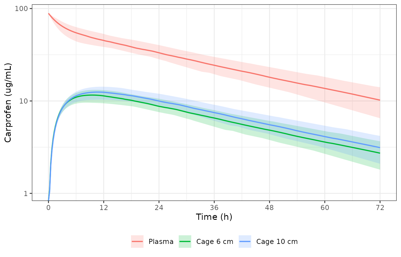

Simulated between-animal variability in plasma and tissue-cage carprofen (median with 5th-95th percentile ribbon, 100 sheep).

c0_cohort <- sim |> dplyr::filter(time == 0) |> dplyr::pull(Cc)
cl_cohort <- sim |> dplyr::filter(time == 0) |> dplyr::pull(cl)

# Vc has essentially no IIV, so C0 is nearly deterministic across the cohort.
stopifnot(abs(median(c0_cohort) / (DOSE_MGKG / vc_raw) - 1) < 0.01)
# CL carries a 13% CV: assert on the centre and a robust quantile, never on
# the extremes of a random cohort (those are not reproducible across rxode2
# builds or solver thread counts).
stopifnot(
  abs(median(cl_cohort) / cl_raw - 1) < 0.05,
  quantile(abs(cl_cohort / cl_raw - 1), 0.9) < 0.35
)

Assumptions and deviations

Residual error is not reported and is fixed to zero. Supplementary Table S1 contains only fixed effects and random-effect standard deviations; it has no error-model rows, and the article body gives no residual-error parameter. The upstream Munn 2022 Table 3 does report a proportional error model (b1 = 0.136 for plasma, b2 = 0.468 for tissue cage), but those are estimates from a different dataset and are deliberately not imported. propSd, propSd_Ccage6 and propSd_Ccage10 are therefore fixed(0), which makes these models typical-value / IIV-only simulators. Anyone needing a residual-error term must supply one.
The structural model is inherited from Munn 2022. Munn 2024 Methods 2.2 describes the fit only as “a custom model as previously described (16)”. The two-compartment plasma model, the negligible-mass cage coupling, and the fact that the cage does not alter the central compartment all come from Munn 2022’s Results and Figure 1, not from the 2024 article.
Cage-size coefficients are applied on the log scale, not additively. Justified above: the additive reading gives a negative k13, and the log reading reproduces Munn 2022 Table 5 across 0-18 cm.
Cage size is encoded as categorical (6 cm reference), following Supplementary Table S1, although Methods 2.2 describes it as a continuous per-cm regressor. With only two cage sizes the two forms are equivalent in fit; the 0* reference row is decisive for how the printed coefficient must be applied.
Two cage states rather than one cage plus a covariate column. Each sheep carried a 6 cm and a 10 cm cage simultaneously, so both are solved together and the cage-size effect is a structural difference between two states rather than a subject-level covariate. No covariate data column is required, and covariateData is empty.
cage6 / cage10 are declared as paper_specific_compartments, not mapped to the canonical isf compartment. The paper’s own Conclusion states that “tissue cage-derived samples are less likely to represent true physiological spaces than samples obtained by ultrafiltration”, so labelling the cage as interstitial fluid would misstate the source.
Per-kilogram parameterisation. Vc (L/kg), CL (L/h/kg) and the dose (mg/kg) are all weight-normalised in the source, so the models are coded on a per-kg basis and no body-weight covariate is used. central / vc is mg/L, which equals ug/mL.
No ultrafiltration compartment. The ultrafiltration arm produced too few quantifiable samples to model (Results 3.1), so it contributes no structure. Moxidectin itself is likewise not a state: it is an analytical correction factor, held at a pseudo-steady state (plasma mean 8.55-8.57 ng/mL, CV 0.05-0.15 within animal), not a modelled analyte.
Vc and k21 between-animal variability is numerically zero and unidentifiable (RSE 1.8e+7% and 2.7e+7%). The reported values are kept so the model states what the paper states, but they should be read as “no detectable variability”, not as estimates.
The authors caution against external use of these estimates. The Discussion states the estimates “allow comparisons within this study, but are unlikely to be as externally valid as in our previous report (16) and therefore are not relied on; the estimation of pharmacokinetic indices was not an objective of this study”. Users wanting a carprofen tissue-cage model for extrapolation should prefer the Munn 2022 parameterisation, which used five cage sizes and reports a residual-error model.
Figure 1 confidence intervals are reconstructed as Wald intervals from the standard errors in Supplementary Table S1. The article generated its intervals with Rsmlx, which may use a different method, so the reconstruction matches the figure’s content and conclusion but not necessarily its exact interval endpoints.