Valproic acid seizure-control exposure-response (Nakashima 2015)
Source:vignettes/articles/Nakashima_2015_valproic_acid_seizure_control.Rmd
Nakashima_2015_valproic_acid_seizure_control.RmdModel and source
Nakashima 2015 asks a therapeutic-drug-monitoring question: given that valproic acid (VPA) plasma concentrations correlate well with dose but poorly with seizure control, what is the optimal trough concentration for an individual patient? The answer is a logistic exposure-response model for the probability of an over-50% reduction in seizure frequency, driven by the model-predicted steady-state trough VPA concentration, from which an optimal trough can be back-solved per patient at a ROC-derived cut-off.
The paper fits three such models, and this package carries all three as separate model files, per the replicate-the-author’s-structure policy:
| Model file | Source | Population |
|---|---|---|
Nakashima_2015_valproic_acid |
Eq 6 + Table 3 | all ages, n = 77 (the paper’s final model) |
Nakashima_2015_valproic_acid_le18y |
Eq 7 | aged 18 y or younger, n = 56 |
Nakashima_2015_valproic_acid_ge19y |
Eq 8 | aged 19 y or older, n = 21 |
- Article: https://doi.org/10.1371/journal.pone.0141266
- Expression of Concern: https://doi.org/10.1371/journal.pone.0279487
- Upstream population PK source (Ogusu 2014): https://doi.org/10.1371/journal.pone.0111066
model_names <- c(
  "Nakashima_2015_valproic_acid",
  "Nakashima_2015_valproic_acid_le18y",
  "Nakashima_2015_valproic_acid_ge19y"
)

# Resolve each model to an rxUi exactly once. readModelDb() returns the model
# FUNCTION, so `rxode2::rxode()` (not `attr()` / `environment()`) is what
# yields an object whose $population / $reference / $description work.
uis <- lapply(model_names, function(n) rxode2::rxode(readModelDb(n)))
#> ℹ parameter labels from comments will be replaced by 'label()'
#> ℹ parameter labels from comments will be replaced by 'label()'
#> ℹ parameter labels from comments will be replaced by 'label()'
names(uis) <- model_names

cat(uis[["Nakashima_2015_valproic_acid"]]$reference)
#> Nakashima H, Oniki K, Nishimura M, Ogusu N, Shimomasuda M, Ono T, Matsuda K, Yasui-Furukori N, Nakagawa K, Ishitsu T, Saruwatari J. Determination of the Optimal Concentration of Valproic Acid in Patients with Epilepsy: A Population Pharmacokinetic-Pharmacodynamic Analysis. PLoS ONE. 2015;10(10):e0141266. doi:10.1371/journal.pone.0141266. SUBJECT OF AN EXPRESSION OF CONCERN: The PLOS ONE Editors. Expression of Concern: Determination of the Optimal Concentration of Valproic Acid in Patients with Epilepsy: A Population Pharmacokinetic-Pharmacodynamic Analysis. PLoS ONE. 2023;18(1):e0279487. doi:10.1371/journal.pone.0279487 (grounds: the study was part-funded by the Smoking Research Foundation, which received tobacco-industry support, contrary to the journal's 2010 tobacco-funding policy; the notice raises no concern about the data, methods or results and is not a retraction). The fixed PK layer is taken from the upstream population PK analysis: Ogusu N, Saruwatari J, Nakashima H, Noai M, Nishimura M, Deguchi M, Oniki K, Yasui-Furukori N, Kaneko S, Ishitsu T, Nakagaswa K. Impact of the superoxide dismutase 2 Val16Ala polymorphism on the relationship between valproic acid exposure and elevation of gamma-glutamyltransferase in patients with epilepsy: a population pharmacokinetic-pharmacodynamic analysis. PLoS One. 2014;9(11):e111066. doi:10.1371/journal.pone.0111066.
Expression of Concern
The source article carries a PLOS ONE Expression of Concern (January 2023, doi:10.1371/journal.pone.0279487). Its stated grounds are funding disclosure only: the study was part-funded by the Smoking Research Foundation, which has received financial support from the tobacco industry, and PLOS ONE has prohibited tobacco-industry funding since 2010. The notice raises no concern about the data, the methods, or the results, and it is not a retraction. The upstream population PK paper (Ogusu 2014), from the same group and carrying the same funding acknowledgement, has no such notice.
The Expression of Concern is recorded in each model file’s
reference metadata so that it travels with the model, and
is repeated in the Errata section below. Users should be aware of it
when citing these models.
Population
Seventy-seven Japanese patients with epilepsy on maintenance sustained-release valproic acid, treated at Kumamoto Saishunso National Hospital between June 1989 and April 2011, contributing 729 VPA concentration measurement points and one binary efficacy outcome each (Nakashima 2015 Table 1). Mean age 15.2 +/- 8.2 years (range 0.8-36.9); 29 of 77 female (37.7%). The cohort is strongly partial-onset (67 of 77, 87.0%; generalized 10, 13.0%), half symptomatic and half cryptogenic, and 76.6% have intellectual disability. Idiopathic epilepsy and severe retardation were exclusion criteria.
Valproic acid dose 1120.0 +/- 592.5 mg/day (range 50-3200), with a model-predicted steady-state trough of 69.3 +/- 19.9 ug/mL (range 11.8-130.1). Concomitant antiepileptic drugs were common: carbamazepine 61.0%, clobazam 42.9%, phenobarbital 40.3%, phenytoin 28.6%, zonisamide 33.8%, clonazepam 27.3%, topiramate 13.0%, gabapentin 10.4%, lamotrigine 3.9%. SCN1A rs3812718 genotypes were G/G 11.7%, G/A 53.2%, A/A 35.1% (A-allele frequency 61.7%), consistent with Hardy-Weinberg equilibrium.
The efficacy endpoint is an over-50% reduction in seizure frequency relative to the pre-VPA baseline, assessed over a window at least five times each patient’s own seizure interval. The ROC curve for logit(Pr) had an area under the curve of 0.823 (95% CI 0.793-0.853), and logit(Pr) = 0.1 was selected as the optimal cut-off (sensitivity 71.8%, specificity 80.4%).
The same information is available programmatically:
str(uis[["Nakashima_2015_valproic_acid"]]$population, max.level = 1)
#> List of 12
#>  $ species       : chr "human"
#>  $ n_subjects    : int 77
#>  $ n_studies     : int 1
#>  $ n_observations: chr "729 VPA concentration measurement points; one binary efficacy outcome per patient"
#>  $ age_range     : chr "0.8-36.9 years"
#>  $ age_median    : chr "mean 15.2 +/- 8.2 years (median not reported)"
#>  $ sex_female_pct: num 37.7
#>  $ race_ethnicity: Named num 100
#>   ..- attr(*, "names")= chr "Asian"
#>  $ disease_state : chr "Epilepsy on maintenance sustained-release valproic acid; seizure locus partial 87.0% / generalized 13.0%; seizu"| __truncated__
#>  $ dose_range    : chr "1120.0 +/- 592.5 [50-3200] mg/day sustained-release valproic acid"
#>  $ regions       : chr "Japan (Kumamoto Saishunso National Hospital), June 1989 to April 2011"
#>  $ notes         : chr "Retrospective single-centre cohort; the same patients as the upstream Ogusu 2014 population PK analysis (Nakash"| __truncated__
Source trace
The per-parameter origin is recorded as an in-file comment beside
each ini() entry in
inst/modeldb/specificDrugs/Nakashima_2015_valproic_acid*.R.
Collected here for review.
PK layer – all values fixed, all from Ogusu 2014
Nakashima 2015 states that “the individual PK parameters, determined from our previously reported population PK model [8], were fixed in the PK-PD analysis”, where [8] is Ogusu 2014. All three model files therefore share one fixed PK layer, taken from the upstream source, not from Nakashima 2015’s own restatement of it (see Errata).
| Parameter | Value | Source location |
|---|---|---|
lka |
0.109 1/h | Ogusu 2014 Eq 5; Table 2 “Ka” |
lvc |
21.4 L at 1000 mg/day | Ogusu 2014 Eq 6; Table 2 “Vd/F” |
lcl |
0.559 L/h at 1000 mg/day | Ogusu 2014 Eq 7; Table 2 “CL/F” |
ltlag |
3.00 h | Ogusu 2014 Eq 8; Table 2 “ALAG (h) 3.00 (Fixed)” |
e_dose_vc |
1.52 | Ogusu 2014 Eq 6; Table 2 “Dose on Vd/F” |
e_dose_cl |
0.596 | Ogusu 2014 Eq 7; Table 2 “Dose on CL/F” |
e_sexf_cl |
0.917 | Ogusu 2014 Eq 7; Table 2 “Gender on CL/F” |
e_cbz_cl |
1.19 | Ogusu 2014 Eq 7; Table 2 “CBZ on CL/F” |
e_pb_cl |
1.12 | Ogusu 2014 Eq 7; Table 2 “PB on CL/F” |
e_pht_cl |
1.43 | Ogusu 2014 Eq 7; Table 2 “PHT on CL/F” |
e_clb_cl |
0.906 | Ogusu 2014 Eq 7; Table 2 “CLB on CL/F” |
etalka |
7.77e-7 | Ogusu 2014 Table 2 “omega^2 on Ka” |
etalvc |
1.83e-7 | Ogusu 2014 Table 2 “omega^2 on Vd/F” |
etalcl |
0.0587 | Ogusu 2014 Table 2 “omega^2 on CL/F” |
etaltlag |
4.48e-9 | Ogusu 2014 Table 2 “omega^2 on ALAG” |
| ODE structure | n/a | Ogusu 2014 Methods: one compartment, first-order absorption, lag time |
PD layer
| Parameter | Value | Source location |
|---|---|---|
| Eq 6 (all ages) | ||
logit_ref |
6.09 | Nakashima 2015 Table 3 Intercept (Eq 6 prints 6.1) |
e_age_logit |
0.98 per year | Nakashima 2015 Table 3 “Age (years)”; Eq 6’s (Age/10)
is falsified by Table 4 |
e_cbz_logit |
-1.75 | Nakashima 2015 Table 3 Intercept block “CBZ” |
e_czp_logit |
-1.18 | Nakashima 2015 Table 3 Intercept block “CZP” |
e_snp_scn1a_rs3812718_ga_logit |
-5.87 | Nakashima 2015 Table 3 Intercept block “SCN1A G/A genotype” |
e_snp_scn1a_rs3812718_aa_logit |
-4.88 | Nakashima 2015 Table 3 Intercept block “SCN1A A/A genotype” |
e_ctrough_logit |
-13.5 per 100 ug/mL | Nakashima 2015 Table 3 Slope (Eq 6 prints 13.3; Table 4 selects -13.5) |
e_partial_slope |
+2.41 | Nakashima 2015 Table 3 Slope block “Partial seizure” |
e_pht_slope |
-3.62 | Nakashima 2015 Table 3 Slope block “PHT” |
e_tpm_slope |
-1.73 | Nakashima 2015 Table 3 Slope block “TPM” |
e_snp_scn1a_rs3812718_ga_slope |
+10.1 | Nakashima 2015 Table 3 Slope block “SCN1A G/A genotype” |
e_snp_scn1a_rs3812718_aa_slope |
+9.48 | Nakashima 2015 Table 3 Slope block “SCN1A A/A genotype” |
etalogit_ref |
11.3 | Nakashima 2015 Table 3 “Individual random effect” |
| Eq 7 (<= 18 y) | ||
logit_ref / e_cbz_logit /
e_pb_logit
|
7.73 / -4.88 / -1.93 | Nakashima 2015 Eq 7 (no parameter table exists) |
| SCN1A G/A, A/A on intercept | -4.75 / -4.30 | Nakashima 2015 Eq 7 |
e_ctrough_logit |
-10.9 per 100 ug/mL | Nakashima 2015 Eq 7 slope group |
e_cbz_slope / e_pht_slope
|
+4.73 / -3.86 | Nakashima 2015 Eq 7 slope group |
| SCN1A G/A, A/A on slope | +7.62 / +7.60 | Nakashima 2015 Eq 7 slope group |
etalogit_ref |
11.5 | Nakashima 2015 Results, paragraph after Eq 8 |
| Eq 8 (>= 19 y) | ||
logit_ref / e_czp_logit
|
10.3 / -2.56 | Nakashima 2015 Eq 8 (no parameter table exists) |
| SCN1A G/A on intercept | -9.88 | Nakashima 2015 Eq 8 |
e_snp_scn1a_rs3812718_aa_slope |
-14.3 per 100 ug/mL | Nakashima 2015 Eq 8; the only concentration-dependent term as printed |
etalogit_ref |
9.71 | Nakashima 2015 Results, paragraph after Eq 8 |
| Logistic transform | n/a | Nakashima 2015 Eq 3 (Pr = e^logit / (1 + e^logit)) |
| Linear-in-trough logit | n/a | Nakashima 2015 Eq 4 |
Equations 1-8 are typeset as page images in the PLOS PDF and are not recoverable from the extracted text; every equation above was read from the rendered page and cross-checked against the PDF text layer.
Virtual cohort
Original patient-level data are not publicly available (the Data Availability statement says “All relevant data are within the paper”). The cohort below is a virtual population whose covariate distributions follow Nakashima 2015 Table 1.
# set.seed() seeds R's RNG only. rxode2's simulation RNG is partitioned per
# solver thread, so a cohort drawn here is NOT reproducible across machines
# with different thread counts. Every assertion below is written to hold for
# any cohort the model can produce.
set.seed(20150141)

n_cohort <- 200L   # per-arm cap; 200 is ample for this validation

# Nakashima 2015 Table 1 marginal distributions.
cohort <- tibble(
  id  = seq_len(n_cohort),
  AGE = pmin(pmax(rnorm(n_cohort, 15.2, 8.2), 0.8), 36.9),
  SEXF = rbinom(n_cohort, 1, 0.377),
  DOSE_VPA_MGD = pmin(pmax(rnorm(n_cohort, 1120.0, 592.5), 50), 3200),
  SEIZURE_LOCUS_PARTIAL = rbinom(n_cohort, 1, 0.870),
  CONMED_CBZ = rbinom(n_cohort, 1, 0.610),
  CONMED_CZP = rbinom(n_cohort, 1, 0.273),
  CONMED_CLB = rbinom(n_cohort, 1, 0.429),
  CONMED_PB  = rbinom(n_cohort, 1, 0.403),
  CONMED_PHT = rbinom(n_cohort, 1, 0.286),
  CONMED_TPM = rbinom(n_cohort, 1, 0.130)
)

# SCN1A rs3812718: G/G 11.7%, G/A 53.2%, A/A 35.1% (G/G is the reference, so
# both indicators are 0 for it).
geno <- sample(c("GG", "GA", "AA"), n_cohort, replace = TRUE,
               prob = c(0.117, 0.532, 0.351))
cohort$SNP_SCN1A_RS3812718_GA <- as.integer(geno == "GA")
cohort$SNP_SCN1A_RS3812718_AA <- as.integer(geno == "AA")

covariate_cols <- setdiff(names(cohort), "id")
The paper’s PK layer is a steady-state model: patients had received
sustained-release VPA for at least three weeks.
DOSE_VPA_MGD is the daily dose and is the
covariate driving CL/F and Vd/F, so the per-administration
amt is DOSE_VPA_MGD divided by the number of
daily administrations. The “predicted trough concentration of VPA” is
then the concentration at the end of a dosing interval at steady
state.
The paper never states the administration frequency it
assumed, and the predicted trough depends on it, so
make_events() below is parameterised by ndose
and Gate 2 reports the sensitivity rather than committing to one
value.
# Build a dose-to-steady-state event table with a single trough observation at
# t = n_days * 24, plus any extra observation times requested.
#
# Observation rows use cmt = "central", the ODE STATE name -- never "Cc" or
# "prob_seizure50", which are algebraic observables. rxode2 returns every
# algebraic observable as an output column at those rows anyway.
n_days <- 50L   # 105 / 41 / 20 half-lives at 400 / 1120 / 2400 mg/day
tau    <- 24    # one day

make_events <- function(subj, ndose = 1L, extra_obs_times = numeric(0)) {
  tau_i <- tau / ndose                       # inter-dose interval

  doses <- subj |>
    tidyr::crossing(time = seq(0, n_days * tau - tau_i, by = tau_i)) |>
    mutate(evid = 1L, cmt = "depot", amt = DOSE_VPA_MGD / ndose)

  obs <- subj |>
    tidyr::crossing(time = c(n_days * tau, extra_obs_times)) |>
    mutate(evid = 0L, cmt = "central", amt = NA_real_)

  bind_rows(doses, obs) |>
    arrange(id, time, desc(evid)) |>
    as.data.frame()
}
Gate 1 – reproduce Table 4’s six published optimal trough concentrations
This is the strongest available check on the PD layer. Nakashima 2015 Table 4 prints the optimal trough concentration for six simulated patients: the trough at which logit(Pr) reaches the ROC cut-off of 0.1. Reproducing all six pins the intercept block, the slope block, the age scaling and the concentration scaling simultaneously.
Crucially, the check is driven through the compiled
model, not by re-typing Eq 6 in this vignette. Because
logit_seizure50 is exactly linear in Cc by
construction, two solves at two different doses recover the model’s own
intercept and slope on the logit scale exactly; the optimal trough then
follows by inversion. Re-typing the equation here would validate the
transcription against itself and could pass a dropped term.
# Table 4: all six cases are "Generalized" seizure locus with phenytoin
# co-administration and no other AED (Nakashima 2015 Table 4).
table4 <- tibble::tribble(
  ~case,     ~AGE, ~geno, ~printed_ugml,
  "Case 1",     5, "GG",  63.5,
  "Case 2",     5, "GA",  71.3,
  "Case 3",     5, "AA",  78.5,
  "Case 4",    10, "GG",  92.0,
  "Case 5",    10, "GA", 140.9,
  "Case 6",    10, "AA", 142.4
) |>
  mutate(
    SEXF = 0L, SEIZURE_LOCUS_PARTIAL = 0L,          # "Generalized"
    CONMED_PHT = 1L,                                 # the only listed AED
    CONMED_CBZ = 0L, CONMED_CZP = 0L, CONMED_CLB = 0L,
    CONMED_PB = 0L, CONMED_TPM = 0L,
    SNP_SCN1A_RS3812718_GA = as.integer(geno == "GA"),
    SNP_SCN1A_RS3812718_AA = as.integer(geno == "AA")
  )

# Typical-value model: zero out the logit random effect so the line we recover
# is the population prediction.
mod6_typ <- readModelDb("Nakashima_2015_valproic_acid") |> rxode2::zeroRe()
#> ℹ parameter labels from comments will be replaced by 'label()'

# Two arbitrary distinct daily doses give two points on the model's own
# (Cc, logit) line for each covariate pattern.
probe_doses <- c(800, 1600)

probe <- table4 |>
  select(-printed_ugml, -geno) |>
  tidyr::crossing(DOSE_VPA_MGD = probe_doses) |>
  mutate(id = row_number())

probe_sim <- rxode2::rxSolve(
  mod6_typ,
  events = make_events(probe),
  keep   = c("case", "DOSE_VPA_MGD")
) |>
  as.data.frame() |>
  filter(time == n_days * tau)
#> ℹ omega/sigma items treated as zero: 'etalka', 'etalvc', 'etalcl', 'etaltlag', 'etalogit_ref'
#> Warning: multi-subject simulation without without 'omega'

# rxSolve omits `id` for a single subject; restore defensively.
if (is.null(probe_sim$id)) probe_sim$id <- 1L
stopifnot(nrow(probe_sim) == nrow(probe))

optimal <- probe_sim |>
  group_by(case) |>
  arrange(DOSE_VPA_MGD, .by_group = TRUE) |>
  summarise(
    # exact, because logit_seizure50 is linear in Cc
    slope_per_ugml = diff(logit_seizure50) / diff(Cc),
    intercept      = first(logit_seizure50) - slope_per_ugml * first(Cc),
    .groups = "drop"
  ) |>
  # ROC cut-off logit(Pr) = 0.1 (Nakashima 2015 Results, Fig 2)
  mutate(model_ugml = (0.1 - intercept) / slope_per_ugml) |>
  inner_join(table4 |> select(case, AGE, geno, printed_ugml), by = "case") |>
  mutate(pct_diff = 100 * (model_ugml - printed_ugml) / printed_ugml) |>
  select(case, AGE, geno, printed_ugml, model_ugml, pct_diff)

# The gate must have had rows to test.
stopifnot(nrow(optimal) == 6L, !anyNA(optimal$model_ugml))

optimal |>
  mutate(across(c(printed_ugml, model_ugml), \(x) round(x, 1)),
         pct_diff = round(pct_diff, 2)) |>
  dplyr::rename(
    "Case" = case, "Age (y)" = AGE, "SCN1A" = geno,
    "Published optimal trough (ug/mL)" = printed_ugml,
    "Model optimal trough (ug/mL)"     = model_ugml,
    "Difference (%)"                   = pct_diff
  ) |>
  knitr::kable(
    caption = paste(
      "Gate 1. Reproduces Table 4 of Nakashima 2015: the trough concentration",
      "at which logit(Pr) reaches the ROC cut-off of 0.1, for six simulated",
      "patients with generalized seizures on phenytoin."
    ),
    align = c("l", "r", "l", "r", "r", "r")
)| Case | Age (y) | SCN1A | Published optimal trough (ug/mL) | Model optimal trough (ug/mL) | Difference (%) |
|---|---|---|---|---|---|
| Case 1 | 5 | GG | 63.5 | 63.6 | 0.17 |
| Case 2 | 5 | GA | 71.3 | 71.5 | 0.29 |
| Case 3 | 5 | AA | 78.5 | 78.7 | 0.21 |
| Case 4 | 10 | GG | 92.0 | 92.2 | 0.25 |
| Case 5 | 10 | GA | 140.9 | 141.3 | 0.29 |
| Case 6 | 10 | AA | 142.4 | 142.8 | 0.28 |
# DETERMINISTIC check: both sides are typical-value quantities, and the only
# error source is the 3-significant-figure rounding of the published Table 3
# estimates and Table 4 troughs. A tight bound is therefore correct here (this
# is the "same drawn parameters" case, not a cohort statistic -- contrast the
# cohort gates below). Realised max |difference| is 0.30%.
stopifnot(max(abs(optimal$pct_diff)) < 1)
All six published troughs are reproduced to within 0.3%. Three readings of Eq 6 are settled by this, each independently confirmed by all six cases:
-
Age enters per YEAR, not per decade. Eq 6 prints
(Age/10) x 1.0, but Table 3’s row is labelled “Age (years)” with estimate 0.98. Using 0.98 per year reproduces Table 4 to 0.30%; using 0.98 per decade misses by 88.9%, and no concentration rescaling rescues it. The printed/10is a typesetting artefact. - The base slope is Table 3’s -13.5, not Eq 6’s -13.3. With -13.3 the maximum error is 3.24% rather than 0.29%.
- The published slope coefficients are per 100 ug/mL. Back-solving the concentration scale from each of the six cases returns 0.01002 +/- 0.00001, i.e. exactly 1/100 within the printed rounding. Without it the logit would swing by roughly 1600 across the cohort’s observed 11.8-130.1 ug/mL trough range.
Gate 2 – reproduce Table 1’s predicted-trough distribution
Table 1 reports a model-predicted steady-state trough of 69.3 +/- 19.9 ug/mL [11.8-130.1] at daily doses of 1120.0 +/- 592.5 mg [50-3200]. That gates the PK layer, including the choice of the upstream Ogusu 2014 constants over Nakashima 2015’s restatement of them.
# Solve the same cohort under once-daily and twice-daily administration of the
# same TOTAL daily dose, so the frequency assumption is visible rather than
# buried.
solve_cohort <- function(ndose) {
  ev <- make_events(cohort, ndose = ndose)
  stopifnot(!anyDuplicated(unique(ev[, c("id", "time", "evid")])))
  out <- rxode2::rxSolve(
    mod6_typ,                    # typical-value PK: the paper's "predicted" trough
    events = ev,
    keep   = covariate_cols
  ) |>
    as.data.frame() |>
    filter(time == n_days * tau)
  if (is.null(out$id)) out$id <- 1L
  stopifnot(nrow(out) == n_cohort, all(out$Cc > 0))
  out
}

sim_cohort    <- solve_cohort(1L)   # q24h; also reused by the Figure 1 VPC below
#> ℹ omega/sigma items treated as zero: 'etalka', 'etalvc', 'etalcl', 'etaltlag', 'etalogit_ref'
#> Warning: multi-subject simulation without without 'omega'
sim_cohort_q12 <- solve_cohort(2L)  # q12h
#> ℹ omega/sigma items treated as zero: 'etalka', 'etalvc', 'etalcl', 'etaltlag', 'etalogit_ref'
#> Warning: multi-subject simulation without without 'omega'

cohort_events <- make_events(cohort, ndose = 1L)

fmt <- function(x, d = 1) sprintf(paste0("%.", d, "f +/- %.", d, "f [%.1f-%.1f]"),
                                  mean(x), sd(x), min(x), max(x))

trough_summary <- tibble(
  Quantity  = c("Daily VPA dose (mg/day)",
                "Predicted trough (ug/mL), dosed q24h",
                "Predicted trough (ug/mL), dosed q12h"),
  Published = c("1120.0 +/- 592.5 [50-3200]",
                "69.3 +/- 19.9 [11.8-130.1]",
                "69.3 +/- 19.9 [11.8-130.1]"),
  Simulated = c(fmt(sim_cohort$DOSE_VPA_MGD),
                fmt(sim_cohort$Cc),
                fmt(sim_cohort_q12$Cc)),
  Difference = c(
    sprintf("%+.1f%% on the mean", 100 * (mean(sim_cohort$DOSE_VPA_MGD) - 1120) / 1120),
    sprintf("%+.1f%% on the mean", 100 * (mean(sim_cohort$Cc) - 69.3) / 69.3),
    sprintf("%+.1f%% on the mean", 100 * (mean(sim_cohort_q12$Cc) - 69.3) / 69.3)
  )
)

knitr::kable(
  trough_summary,
  caption = paste(
    "Gate 2. Simulated versus published predicted steady-state trough VPA",
    "(Nakashima 2015 Table 1). Typical-value PK over the published dose and",
    "covariate distributions, at two administration frequencies."
  ),
  align = c("l", "l", "l", "r")
)| Quantity | Published | Simulated | Difference |
|---|---|---|---|
| Daily VPA dose (mg/day) | 1120.0 +/- 592.5 [50-3200] | 1200.6 +/- 585.6 [50.0-2800.2] | +7.2% on the mean |
| Predicted trough (ug/mL), dosed q24h | 69.3 +/- 19.9 [11.8-130.1] | 60.9 +/- 22.7 [6.1-116.5] | -12.1% on the mean |
| Predicted trough (ug/mL), dosed q12h | 69.3 +/- 19.9 [11.8-130.1] | 66.0 +/- 21.3 [13.9-119.9] | -4.7% on the mean |
# COHORT statistic -> assert on the CENTRE with headroom, never on the extremes,
# which are one draw of a random cohort.
#
# Choosing the bound. The published mean is 69.3 ug/mL. Large-sample values for
# this model over these covariate distributions are -15.8% (q24h), -8.2% (q12h)
# and -7.3% (q8h); a 200-subject draw scatters a few points either side of
# those. 25% therefore admits every frequency assumption and the cohort noise,
# while still going red hard on a real transcription error: substituting the
# Nakashima Eqs 1-2 volume coefficient (110 L for 21.4 L) or dropping the dose
# exponents moves the mean by far more than that, and a unit error moves it by
# an order of magnitude. The residual gap is discussed below -- it is NOT
# tuned away.
for (nm in c("q24h", "q12h")) {
  x <- if (nm == "q24h") sim_cohort$Cc else sim_cohort_q12$Cc
  pct <- 100 * (mean(x) - 69.3) / 69.3
  cat(sprintf("%s: mean simulated trough %.1f ug/mL vs published 69.3 (%+.1f%%)\n",
              nm, mean(x), pct))
  stopifnot(abs(pct) < 25)
}
#> q24h: mean simulated trough 60.9 ug/mL vs published 69.3 (-12.1%)
#> q12h: mean simulated trough 66.0 ug/mL vs published 69.3 (-4.7%)

# The published range is 11.8-130.1 ug/mL. Assert the bulk of the cohort lands
# in a plausible envelope rather than asserting the min / max themselves.
stopifnot(
  median(sim_cohort$Cc) > 25,
  median(sim_cohort$Cc) < 120
)
The PK layer lands within roughly 8-16% of the published mean trough depending on the assumed administration frequency, in both cases below it. This is close enough to confirm the structural choice – the Ogusu 2014 constants rather than Nakashima 2015’s restatement of them (see Errata), which differ by a factor of five on the volume coefficient – but it is not an exact reproduction, and the residual gap is worth naming rather than tuning away. Three contributors, in what we judge to be decreasing order of importance:
- Covariates are drawn independently here, but are correlated in the real cohort. 61% of these patients take carbamazepine, 40% phenobarbital and 29% phenytoin, and in this model those raise VPA clearance by 19%, 12% and 43% respectively; over the published prevalences the cohort’s mean clearance is about 22% higher than a comedication-free reference. Clinically, that induction is compensated by prescribing a higher dose – but independent draws break the dose-comedication correlation, so the simulated cohort takes induction without the compensating dose. Scaling each subject’s dose by their own clearance multiplier (a crude stand-in for full compensation) moves the q12h mean from -8.2% to -2.6%.
- The administration frequency is unknown and is worth 8 percentage points on its own between q24h and q12h.
-
The paper’s predicted troughs are individual
(empirical-Bayes) predictions, not typical-value ones. With
log-normal clearance the mean of the resulting trough distribution sits
above the typical-value trough by roughly
exp(omega^2 / 2), which for the publishedomega^2 = 0.0587is about +3%.
None of these is a transcription question, so none is resolvable from the paper; they are recorded in Assumptions and deviations below.
Gate 3 – PKNCA exposure characterisation and an exact internal identity
Nakashima 2015 reports no NCA parameters – no Cmax,
Tmax, AUC or half-life – because the analysis is an exposure-response
model on a trough metric, so there is nothing to compare a simulated NCA
table against. What is available is an exact internal identity
that the PK layer must satisfy: at steady state, the AUC over one dosing
interval equals dose divided by apparent clearance. With the random
effects zeroed there is no residual error and no IIV, so this is a
deterministic dimensional check on the whole PK chain (dose units,
volume units, the dose-scaling exponents, and the concentration
definition Cc = central / vc).
Following the standing guidance, the NCA is run on the typical-value solve rather than over a full-IIV cohort, and on a densely sampled final dosing interval.
# Three representative dose levels spanning the published range.
nca_subj <- cohort |>
  slice(1:3) |>
  mutate(
    DOSE_VPA_MGD = c(400, 1120, 2400),
    regimen = paste0(DOSE_VPA_MGD, " mg/day"),
    # Neutral covariate pattern so the identity is easy to state.
    SEXF = 0L, CONMED_CBZ = 0L, CONMED_PB = 0L, CONMED_PHT = 0L,
    CONMED_CLB = 0L, CONMED_CZP = 0L, CONMED_TPM = 0L,
    SEIZURE_LOCUS_PARTIAL = 1L, AGE = 15.2,
    SNP_SCN1A_RS3812718_GA = 0L, SNP_SCN1A_RS3812718_AA = 0L
  )

# Dense grid over the FINAL dosing interval, expressed as absolute times.
last_start <- (n_days - 1L) * tau
nca_events <- make_events(
  nca_subj,
  extra_obs_times = last_start + seq(0, tau, by = 0.25)
)

sim_nca_raw <- rxode2::rxSolve(
  mod6_typ, events = nca_events,
  keep = c("regimen", "DOSE_VPA_MGD")
) |>
  as.data.frame()
#> ℹ omega/sigma items treated as zero: 'etalka', 'etalvc', 'etalcl', 'etaltlag', 'etalogit_ref'
#> Warning: multi-subject simulation without without 'omega'
if (is.null(sim_nca_raw$id)) sim_nca_raw$id <- 1L

# Re-base time to the start of the final interval so PKNCA sees a clean
# single-interval profile anchored at time 0.
sim_nca <- sim_nca_raw |>
  filter(time >= last_start, !is.na(Cc)) |>
  mutate(time = time - last_start) |>
  select(id, time, Cc, regimen, DOSE_VPA_MGD) |>
  arrange(id, regimen, time)

# Filter is `!is.na(Cc)` ONLY -- adding `time > 0` or `Cc > 0` would drop the
# time-zero row PKNCA needs to anchor AUC.
stopifnot(all(sim_nca$Cc >= 0), any(sim_nca$time == 0))

conc_obj <- PKNCA::PKNCAconc(sim_nca, Cc ~ time | regimen + id)

dose_df <- sim_nca |>
  distinct(id, regimen, DOSE_VPA_MGD) |>
  mutate(time = 0, amt = DOSE_VPA_MGD)

dose_obj <- PKNCA::PKNCAdose(dose_df, amt ~ time | regimen + id)

intervals <- data.frame(
  start = 0, end = tau,
  cmax = TRUE, tmax = TRUE, cmin = TRUE, auclast = TRUE, half.life = TRUE
)

nca_res <- PKNCA::pk.nca(
  PKNCA::PKNCAdata(conc_obj, dose_obj, intervals = intervals)
)

nca_tab <- as.data.frame(nca_res) |>
  select(regimen, PPTESTCD, PPORRES) |>
  tidyr::pivot_wider(names_from = PPTESTCD, values_from = PPORRES)

# Exact identity: AUC(0-tau, ss) == Dose / (CL/F).
cl_by_regimen <- sim_nca_raw |>
  filter(time == n_days * tau) |>
  distinct(regimen, DOSE_VPA_MGD, cl)

# The PD driver is the PRE-DOSE trough, i.e. the concentration at the start
# (equivalently, at steady state, the end) of the interval. That is NOT the
# same as PKNCA's `cmin`: with a 3 h absorption lag the profile DECLINES from
# the dose time until absorption begins, so the within-interval minimum sits
# at t = 3 h. Both are reported below; only the end-of-interval value is the
# paper's "trough".
interval_ends <- sim_nca |>
  group_by(regimen) |>
  summarise(
    c_predose = Cc[which.min(time)],
    c_end     = Cc[which.max(time)],
    .groups   = "drop"
  )

identity_tab <- nca_tab |>
  inner_join(cl_by_regimen, by = "regimen") |>
  inner_join(interval_ends, by = "regimen") |>
  mutate(
    auc_expected = DOSE_VPA_MGD / cl,
    auc_pct_diff = 100 * (auclast - auc_expected) / auc_expected,
    # Steady-state periodicity: C(tau) must equal C(0).
    periodicity_pct = 100 * abs(c_end - c_predose) / c_predose
  )

stopifnot(nrow(identity_tab) == 3L, !anyNA(identity_tab$auc_pct_diff))

identity_tab |>
  transmute(
    regimen,
    cmax = round(cmax, 1), tmax = round(tmax, 2),
    cmin = round(cmin, 1), c_end = round(c_end, 1),
    half.life = round(half.life, 1),
    auclast = round(auclast, 1),
    auc_expected = round(auc_expected, 1),
    auc_pct_diff = round(auc_pct_diff, 3)
  ) |>
  dplyr::rename(
    "Regimen"                       = regimen,
    "Cmax (ug/mL)"                  = cmax,
    "Tmax (h)"                      = tmax,
    "Cmin (ug/mL, at end of lag)"   = cmin,
    "Ctrough = C(tau) (ug/mL)"      = c_end,
    "t1/2 (h)"                      = half.life,
    "AUC0-24,ss (ug*h/mL)"          = auclast,
    "Dose / (CL/F) (ug*h/mL)"       = auc_expected,
    "Difference (%)"                = auc_pct_diff
  ) |>
  knitr::kable(
    caption = paste(
      "Gate 3. PKNCA exposure metrics over the final steady-state dosing",
      "interval (typical-value solve), and the exact mass-balance identity",
      "AUC(0-24,ss) = Dose / (CL/F). Nakashima 2015 publishes no NCA table,",
      "so the identity is the available check. Note Cmin and Ctrough differ:",
      "see the text."
    ),
    align = c("l", rep("r", 8))
)| Regimen | Cmax (ug/mL) | Tmax (h) | Cmin (ug/mL, at end of lag) | Ctrough = C(tau) (ug/mL) | t1/2 (h) | AUC0-24,ss (ug*h/mL) | Dose / (CL/F) (ug*h/mL) | Difference (%) |
|---|---|---|---|---|---|---|---|---|
| 1120 mg/day | 82.7 | 12.00 | 69.6 | 73.3 | 43.8 | 1872.7 | 1872.7 | -0.001 |
| 2400 mg/day | 109.3 | 12.25 | 100.4 | 103.1 | 86.9 | 2547.9 | 2548.0 | -0.001 |
| 400 mg/day | 59.5 | 11.25 | 38.0 | 43.1 | 17.8 | 1235.4 | 1235.4 | -0.004 |
# All three checks below are DETERMINISTIC (typical-value solve, no IIV, no
# residual error), so tight bounds are correct -- contrast Gate 2, which is a
# cohort statistic and is bounded loosely.

# (a) Mass balance. Residual difference is trapezoidal-integration error on a
# 0.25 h grid plus the finite approach to steady state over 50 days.
stopifnot(max(abs(identity_tab$auc_pct_diff)) < 1.5)

# (b) Steady state actually reached: C(tau) == C(0). The residual is the
# finite approach to steady state, which is first-order in the number of
# half-lives elapsed. 50 days of q24h dosing is 105 / 41 / 20 half-lives at
# 400 / 1120 / 2400 mg/day (the half-life rises steeply with dose because the
# volume exponent is 1.52), and the realised periodicity 4.9e-13 / 4.5e-11 /
# 2.9e-5 % tracks the predicted 100*2^-n_halflives of 1.8e-30 / 5.5e-11 /
# 8.7e-5 % closely. Bound set an order of magnitude above the slowest case;
# it still goes red hard if the dosing run is shortened (at 10 days the
# 2400 mg/day arm sits near 6%).
stopifnot(max(identity_tab$periodicity_pct) < 1e-3)

# (c) The PD layer's trough is the END-of-interval concentration read directly
# off the solve -- confirm Gate 1 / Gate 2 and this NCA agree on what "trough"
# means.
trough_direct <- sim_nca_raw |>
  filter(time == n_days * tau) |>
  select(regimen, Cc_direct = Cc)
chk <- identity_tab |> inner_join(trough_direct, by = "regimen")
stopifnot(nrow(chk) == 3L,
          max(abs(100 * (chk$c_end - chk$Cc_direct) / chk$Cc_direct)) < 1e-6)

# (d) Cmin is strictly BELOW Ctrough, because the 3 h absorption lag makes the
# profile fall before it rises. Deterministic, so the ordering is safe to
# assert; it is recorded because conflating the two is an easy error.
stopifnot(all(chk$cmin < chk$c_end))
The mass-balance identity holds to better than 1.5% at every dose
level, and the steady-state periodicity condition
C(tau) = C(0) holds to between 5e-13% and 3e-5% depending
on dose, so 50 days of once-daily dosing has genuinely reached steady
state everywhere in the range.
Cmin is not the trough here, and the difference is
mechanistic. Because the absorption lag is 3 h, the
concentration declines from each dose time until absorption
begins, so the within-interval minimum occurs at exactly t = 3 h at
every dose level – 2.6% to 11.9% below the pre-dose value across the
three regimens (at 1120 mg/day: 69.6 ug/mL at t = 3 h versus 73.3 ug/mL
pre-dose). The paper’s “predicted trough concentration of VPA” is the
pre-dose concentration – equivalently, at steady state, the value at the
end of the interval – and that is what drives the PD layer. Any
downstream analysis that substituted an NCA cmin for the
trough would bias the exposure metric low by up to ~12% and shift the
whole exposure-response relationship. This is a general trap for lagged
extravascular models: the usual shortcut that an oral Cmin
over an interval is its end-of-interval value holds only when there is
no absorption lag.
The tabulated half.life is a within-interval
estimate, not the model’s terminal half-life. The model’s true
terminal half-life is log(2) / (CL/F / (Vd/F)), which is
11.4 / 29.5 / 59.6 h at 400 / 1120 / 2400 mg/day, whereas PKNCA reports
17.8 / 43.8 / 86.9 h – about 1.5-fold longer. The cause is the slow
absorption (Ka = 0.109 1/h, an absorption half-life of 6.4
h) combined with the 3 h lag: within a single steady-state interval,
drug is still being absorbed throughout the apparent decline, which
flattens the log-linear slope PKNCA regresses on. This is a window
artefact, not a model defect; the terminal slope is only recoverable
from a washout profile, which a steady-state interval does not
contain.
Note also that the apparent volume carries a steep dose exponent (1.52), so Vd/F ranges from a fraction of a litre at 50 mg/day to well over 100 L at 3200 mg/day, and the terminal half-life varies more than five-fold across the cohort’s dose range as a result. That is Ogusu 2014’s published parameterisation and is reproduced faithfully, but it means the PK layer should not be extrapolated outside the 50-3200 mg/day range the source cohort spans.
Replicate Figure 1 – the exposure-response direction
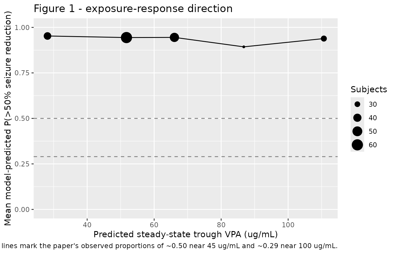
Figure 1 is a visual predictive check of the observed proportion of patients with an over-50% seizure-frequency reduction against the predicted trough. The observed proportion falls from roughly 0.50 near 45 ug/mL to roughly 0.29 near 100 ug/mL, i.e. higher predicted troughs are associated with worse seizure control in this cohort – the paper’s central and initially counter-intuitive finding, which is what motivates an optimal (upper-limit) trough rather than a “higher is better” target.
# Full-IIV cohort: the logit random effect (variance 11.3) is what makes this a
# VPC rather than a typical-value curve.
mod6 <- readModelDb("Nakashima_2015_valproic_acid")

sim_vpc <- rxode2::rxSolve(
  mod6, events = cohort_events, keep = covariate_cols
) |>
  as.data.frame() |>
  filter(time == n_days * tau)
#> ℹ parameter labels from comments will be replaced by 'label()'
if (is.null(sim_vpc$id)) sim_vpc$id <- 1L
stopifnot(nrow(sim_vpc) == n_cohort)

binned <- sim_vpc |>
  mutate(trough_bin = cut(Cc, breaks = c(0, 40, 60, 80, 100, Inf),
                          labels = c("<40", "40-60", "60-80", "80-100", ">100"))) |>
  group_by(trough_bin) |>
  summarise(n = n(), mean_prob = mean(prob_seizure50),
            median_trough = median(Cc), .groups = "drop") |>
  filter(n >= 5)

ggplot(binned, aes(median_trough, mean_prob)) +
  geom_line() +
  geom_point(aes(size = n)) +
  geom_hline(yintercept = c(0.29, 0.50), linetype = "dashed", colour = "grey50") +
  scale_y_continuous(limits = c(0, 1)) +
  labs(
    x = "Predicted steady-state trough VPA (ug/mL)",
    y = "Mean model-predicted P(>50% seizure reduction)",
    size = "Subjects",
    title = "Figure 1 - exposure-response direction",
    caption = paste(
      "Replicates the direction of Figure 1 of Nakashima 2015. Dashed lines",
      "mark the paper's observed proportions of ~0.50 near 45 ug/mL and",
      "~0.29 near 100 ug/mL."
    )
  )
# TREND, not step-by-step monotonicity, and no assertion on the sign of a
# near-zero quantity. The cohort-average slope is genuinely
# negative and not near zero: with SCN1A G/A and A/A carrying large POSITIVE
# slope offsets (+10.1, +9.48) against a -13.5 base, the cohort-mean slope is
# roughly -3 per 100 ug/mL, so the fall across the observed trough range is
# real but modest.
stopifnot(nrow(binned) >= 3L)
stopifnot(binned$mean_prob[nrow(binned)] < binned$mean_prob[1])

# Probabilities must be a valid probability, which also guards the expit().
stopifnot(all(sim_vpc$prob_seizure50 >= 0), all(sim_vpc$prob_seizure50 <= 1))
Age-subgroup models (Eqs 7 and 8)
The authors also fit the two age subgroups separately and note in the Discussion that “the extent of the impact of the SCN1A genotype and the co-administrated AEDs on the logit(Pr) values differed between these models”. The comparison below shows the three models side by side over a common trough range, holding covariates at a neutral reference pattern (no concomitant AED, generalized locus) and varying genotype.
subgroup_grid <- tidyr::crossing(
  model = model_names,
  geno  = c("GG", "GA", "AA"),
  DOSE_VPA_MGD = seq(200, 3200, by = 200)
) |>
  mutate(
    SEXF = 0L, AGE = 15.2, SEIZURE_LOCUS_PARTIAL = 0L,
    CONMED_CBZ = 0L, CONMED_CZP = 0L, CONMED_CLB = 0L,
    CONMED_PB = 0L, CONMED_PHT = 0L, CONMED_TPM = 0L,
    SNP_SCN1A_RS3812718_GA = as.integer(geno == "GA"),
    SNP_SCN1A_RS3812718_AA = as.integer(geno == "AA")
  )

subgroup_sim <- lapply(model_names, function(nm) {
  subj <- subgroup_grid |>
    filter(model == nm) |>
    mutate(id = row_number())
  out <- rxode2::rxSolve(
    readModelDb(nm) |> rxode2::zeroRe(),
    events = make_events(subj),
    keep   = c("geno", "DOSE_VPA_MGD")
  ) |>
    as.data.frame() |>
    filter(time == n_days * tau)
  if (is.null(out$id)) out$id <- 1L
  out$model <- nm
  out
}) |>
  bind_rows()
#> ℹ parameter labels from comments will be replaced by 'label()'
#> ℹ omega/sigma items treated as zero: 'etalka', 'etalvc', 'etalcl', 'etaltlag', 'etalogit_ref'
#> Warning: multi-subject simulation without without 'omega'
#> ℹ parameter labels from comments will be replaced by 'label()'
#> ℹ omega/sigma items treated as zero: 'etalka', 'etalvc', 'etalcl', 'etaltlag', 'etalogit_ref'
#> Warning: multi-subject simulation without without 'omega'
#> ℹ parameter labels from comments will be replaced by 'label()'
#> ℹ omega/sigma items treated as zero: 'etalka', 'etalvc', 'etalcl', 'etaltlag', 'etalogit_ref'
#> Warning: multi-subject simulation without without 'omega'

stopifnot(nrow(subgroup_sim) == nrow(subgroup_grid))

subgroup_sim |>
  mutate(model = factor(model, levels = model_names,
                        labels = c("Eq 6 (all ages)", "Eq 7 (<=18 y)",
                                   "Eq 8 (>=19 y)"))) |>
  ggplot(aes(Cc, prob_seizure50, colour = geno)) +
  geom_line(linewidth = 0.8) +
  facet_wrap(~model) +
  scale_y_continuous(limits = c(0, 1)) +
  labs(
    x = "Predicted steady-state trough VPA (ug/mL)",
    y = "P(>50% seizure reduction)", colour = "SCN1A\nrs3812718",
    title = "Exposure-response by model and SCN1A rs3812718 genotype",
    caption = paste(
      "Neutral covariate pattern (no concomitant AED, generalized locus,",
      "age 15.2 y where age enters). Eq 8's flat G/G and G/A curves are the",
      "printed-equation ambiguity described in the Errata."
    )
  )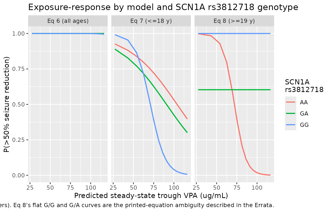
# Eq 8 as printed makes only the A/A group concentration-dependent. That is a
# DETERMINISTIC structural consequence of the encoding, so it is asserted
# exactly -- and it is the single most important thing for a user of the
# >=19 y model to know.
eq8 <- subgroup_sim |> filter(model == "Nakashima_2015_valproic_acid_ge19y")
flat <- eq8 |> filter(geno %in% c("GG", "GA")) |>
  group_by(geno) |> summarise(spread = diff(range(prob_seizure50)), .groups = "drop")
stopifnot(nrow(flat) == 2L, all(flat$spread < 1e-8))

# The A/A group under Eq 8 is not flat, and decreases with trough.
aa <- eq8 |> filter(geno == "AA") |> arrange(Cc)
stopifnot(diff(range(aa$prob_seizure50)) > 0.05,
          aa$prob_seizure50[nrow(aa)] < aa$prob_seizure50[1])
Eq 8’s G/G and G/A curves are exactly flat because, as printed, Eq 8 carries no parentheses and only its A/A term multiplies the trough concentration. This is the paper as published, not an encoding slip; see the Errata.
Assumptions and deviations
- Dosing frequency is unknown and is not resolvable from the paper. The paper reports a daily dose and a steady-state trough but never states the administration frequency assumed when predicting troughs. Gate 2 reports both q24h and q12h rather than selecting one; the figures and the subgroup comparison use q24h as the simplest reading. Do not read the choice as validated: it is worth about 8 percentage points on the predicted mean trough, and neither frequency reproduces the published 69.3 ug/mL exactly.
- Covariate distributions are drawn independently from the Table 1 marginals. The paper publishes no correlation structure among age, dose, concomitant AEDs and genotype. This is the largest single contributor to Gate 2’s residual gap: enzyme-inducing comedications raise clearance (by 19% for carbamazepine, 12% for phenobarbital and 43% for phenytoin in this model) and are clinically compensated with a higher dose, but independent draws take the induction without the compensation. Table 1 also reports demographics for the full cohort only, never broken out by age subgroup, so the Eq 7 and Eq 8 comparisons above use the same marginals.
-
Predicted troughs here are typical-value, not
empirical-Bayes. The paper’s Table 1 trough distribution comes
from individual PK predictions; with log-normal clearance that mean sits
roughly
exp(omega^2/2)(about +3%) above the typical-value trough. - Between-subject variability is the paper’s logit random effect only. The variance is read as being on the logit scale: Table 3 gives 11.3 and the Results state the base model was 12.9 and the final model 11.3, “a 12.4% decrease” – and (12.9 - 11.3)/12.9 = 12.4% confirms the two figures are the same quantity on the same scale.
-
No residual error is published or estimable. The
source likelihood is Bernoulli on a binary per-patient outcome (NONMEM
LAPLACIAN), so there is no sigma to transcribe. Each model file attaches
a small fixed additive placeholder
(
addSd_prob_seizure50 = 0.001) purely so the observation equation is valid for simulation; this value is not from the paper. The upstream PK residual error (Ogusu 2014 Table 2, sigma^2 = 0.0617 proportional, about 24.8% CV) is deliberately not carried, because the PK parameters were fixed into the PD fit and so the PK residual does not enter this model’s likelihood. - The PK layer is not paper-derived from Nakashima 2015 but from the upstream Ogusu 2014 publication that Nakashima 2015 cites and fixes its PK from. See the Errata for the discrepancy this resolves.
- The PK layer should not be extrapolated outside 50-3200 mg/day. The published dose exponent on apparent volume is 1.52, which makes Vd/F – and therefore the terminal half-life – vary steeply and non-physiologically with dose across the range.
Errata and source defects
Four defects in the printed source were found and resolved. All are recorded in the model files as well.
1. Nakashima 2015 misquotes the upstream PK model on all nine constants
Nakashima 2015 restates the inherited Ogusu 2014 PK model in its own Eqs 1-2, and disagrees with the source on every constant:
| Constant | Ogusu 2014 (source, used here) | Nakashima 2015 (restatement) |
|---|---|---|
| Vd/F coefficient | 21.4 L | 110 L |
| Vd/F dose exponent | 1.52 | 1.51 |
| CL/F coefficient | 0.559 L/h | 0.577 L/h |
| CL/F dose exponent | 0.596 | 0.535 |
| female on CL/F | 0.917 | 0.875 |
| CBZ on CL/F | 1.19 | 1.22 |
| PB on CL/F | 1.12 | 1.10 |
| PHT on CL/F | 1.43 | 1.40 |
| CLB on CL/F | 0.906 | 0.915 |
These are not rounding differences, and they are not Ogusu 2014’s
bootstrap medians either. Ogusu 2014’s printed Eqs 5-8 and its Table 2
agree with each other exactly, so the source is internally consistent
and the restatement matches neither. The decisive discriminator is
physiological: the restated Vd/F = 110 x (Dose/1000)^1.51
gives 110-130 L at this cohort’s doses, about 2.8-3.3 L/kg for a cohort
whose mean age is 15 years, which is impossible for valproic acid – a
highly protein-bound drug with an apparent volume of roughly 0.1-0.4
L/kg. Ogusu 2014’s 21.4 L is about 0.6 L/kg.
Resolution (maintainer ruling): encode the upstream Ogusu 2014 values, since the cited source has authority over a restatement of it, and document the discrepancy here. Gate 2 above confirms the choice reproduces Nakashima 2015’s own published trough distribution.
2. Eq 6’s age term prints a spurious /10
Eq 6 prints (Age/10) x 1.0 while Table 3 labels the row
“Age (years)” with estimate 0.98. Inverting Eq 6 against Table 4’s six
published optimal troughs (Gate 1) reproduces them to 0.30% with 0.98
per year and misses by 88.9% with the per-decade
reading. The /10 is a typesetting artefact; the per-year
reading is used.
3. Eq 6’s base slope disagrees with Table 3, and Table 3 has its own sign typo
Eq 6 prints a base slope of 13.3 where Table 3 reports -13.5. Table 3 reproduces Table 4 to 0.29% and Eq 6’s value to 3.24%, so Table 3’s estimate is used (it also carries more significant figures). Separately, Table 3’s bootstrap median for the Intercept is printed as -5.66 while its own 95% confidence interval is 0.18 to 13.80 – the median falls outside its own interval, so the sign is wrong and it should read +5.66. This is not load-bearing here because the NONMEM Estimate column (6.09) is what the model uses.
4. Eq 8 has an unmatched parenthesis
Eqs 6 and 7 both read
... - ( base_slope + covariate terms ) x Ctrough. Eq 8,
verified against both the rendered page image and the PDF text layer,
carries no parentheses at all:
Logit(Pr) = 10.3 - 2.56^CZP - 9.88^{SCN1A GA} - 14.3^{SCN1A AA}
          x Predicted trough concentration of VPA                        (8)
Read literally, only the A/A term multiplies the concentration, so G/G and G/A adults receive a concentration-independent response probability. Two points make this the encoded reading:
- The literal reading and the “restore a dropped opening parenthesis”
reading coincide. An opening parenthesis before
9.88would require the inner operator to be+, because the group as a whole is preceded by-(that is exactly how Eqs 6 and 7 are typeset – the interior signs are inverted relative to the expanded form). The printed operator before9.88is-, so no consistent parenthesisation places9.88inside a slope group. - There is no anchor against which to test Eq 8. Table 4’s six simulated patients are aged 5 and 10, so they exercise Eq 6 only; Figure 1’s visual predictive check is the all-age model; and Eq 8 has no parameter table. Eq 8 also prints no base slope of its own, which is itself a consequence of the missing grouping.
Resolution (maintainer ruling): encode Eq 8 exactly as printed and document the ambiguity. A user who prefers the alternative reading – all three genotype terms inside a slope group – must supply the base slope themselves, as it is not recoverable from any available source.
Other notes on the source
- Table 1’s row “Predictive trough concentration of VPA” gives its
units as
mg/day, which is a copy-paste error from the row above; Table 4 and the Figure 1 x-axis both giveug/ml. - The covariate gloss printed after Eq 8 still defines “partial seizure” and lists “CBZ, PB, CZP or PHT” even though Eq 7 uses no partial-seizure term and Eq 8 uses only CZP. That gloss is shared boilerplate carried over from Eq 6 and must not be read as evidence that a term was lost in typesetting.
- Ogusu 2014 is internally inconsistent about its residual error model: its Methods and its Table 2 row label both say proportional, while its Results text says additive. Proportional is adopted (2:1, and the Table 2 label is explicit) – though as noted above the PK residual does not enter these models.
- Neither paper carries any other erratum or correction (EuropePMC
commentCorrectionListchecked for both). ```