Ethanol and acetaldehyde whole-body PBPK (Zhu 2021)
Source:vignettes/articles/Zhu_2021_ethanol.Rmd
Zhu_2021_ethanol.RmdModel and source
mod_fun <- readModelDb("Zhu_2021_ethanol_pbpk")
ui <- rxode2::rxode2(mod_fun)- Citation: Zhu L, Pei W, Thiele I, Mahadevan R (2021). Integration of a physiologically-based pharmacokinetic model with a whole-body, organ-resolved genome-scale model for characterization of ethanol and acetaldehyde metabolism. PLoS Comput Biol 17(8):e1009110. doi:10.1371/journal.pcbi.1009110. Model code: https://github.com/LMSE/HH-PBPK-Ethanol (commit b14305a). Michaelis-Menten constants from Umulis DM, Guerdjikov NM, Kuchler T, et al. (2005) Alcohol 35(1):3-12, doi:10.1016/j.alcohol.2004.11.004.
- Description: PBPK (whole-body, hand-written MATLAB; dynamic flux-balance coupling to the Harvey genome-scale model reduced to its continuous limit). Ethanol and acetaldehyde disposition after an oral drink in adult men (Zhu 2021 PLoS Comput Biol). Fourteen flow-limited tissues (adipose, arterial blood, brain, small and large intestine, heart, kidney, liver, lung, muscle, pancreas, skin, spleen, stomach) per analyte plus stomach and small-intestine lumens for ethanol. Organ masses, blood flows and cardiac output from age / height / weight / body-fat correlations; partition coefficients from logP, fraction unbound and tissue lipid/water composition. Stomach and small-intestine absorption and stomach-to-SI transit are quadratic functions of the drink ethanol fraction (S2 Text, fitted to Mitchell 2014). Hepatic ADH and ALDH2 and gastric ADH follow Michaelis-Menten kinetics (Umulis 2005 constants) with an age factor on all three. ALDH2 isoform activity (Table 4) and a steady blood disulfiram level (S3 Text) scale hepatic ALDH2. Urine, sweat and breath excretion are the Harvey flux-balance bounds expressed as fixed fractions of the hepatic ADH rate (set them to 0 to recover the base PBPK used for Figs 6-8). Deterministic: no IIV, no residual error. Encoded from the authors’ deposited code, which reproduces Figs 4-8; the printed kSI correlation (S2.3) has a sign typo. Male only. See the vignette.
- Article: https://doi.org/10.1371/journal.pcbi.1009110
- Model code: https://github.com/LMSE/HH-PBPK-Ethanol (commit
b14305a) - Supplements: S1 Text (organ-specific equations), S2 Text (drink-fraction absorption correlations), S3 Text (disulfiram-ALDH2 correlation).
Zhu et al. built a 34-state whole-body PBPK model for ethanol and its
primary metabolite acetaldehyde, and coupled it to the male whole-body
genome-scale metabolic reconstruction Harvey via dynamic
flux-balance analysis (dFBA). The genome-scale layer is used only to set
the boundaries of a handful of excretion and side-metabolism reactions
(urine, sweat, breath, colonic catalase) as fractions of the hepatic
alcohol-dehydrogenase (ADH) rate. In the authors’ deposited simulations
the flux-balance solver holds those excretion reactions at their upper
bounds, so the continuous limit of the coupled model is an ordinary
system of ODEs. That continuous limit is what this package encodes: the
whole-body PBPK, with the genome-scale excretion fractions entered as
fixed multipliers of the hepatic ADH rate. Setting
f_urine_wbm, f_sweat_wbm and
f_breath_wbm to zero recovers the base PBPK (ModelVer 1)
that generated the paper’s Figs 6-8.
The rate constants and the genome-scale linear programme themselves are not part of the packaged model; see Assumptions and deviations for what is and is not reproducible from the published sources.
Population
No new subjects were studied. The model reuses two published clinical
datasets: the gut-absorption correlations (S2 Text) were fitted to the
mean blood-ethanol profiles of Mitchell et al. 2014 (15 men; mean age
37.8 y, 82.66 kg, 177.1 cm, 20% body fat; 0.5 g/kg ethanol as beer, wine
or spirits, Fig 3), and the hepatic Michaelis-Menten constants come from
Umulis et al. 2005, whose model was fitted to Jones et al. 1988 (10
men). Every scenario in Figs 4-8 is a single simulated man of age 25.6
y, 74.5 kg, 180 cm, 20% body fat drinking 0.25 g/kg ethanol. The model
supports men only (main.m: “female (not yet
supported)”).
str(mod_fun()$population)
#> List of 10
#>  $ species       : chr "human"
#>  $ n_subjects    : int 25
#>  $ n_studies     : int 2
#>  $ age_range     : chr "group means only: 37.8 years (Mitchell 2014, n = 15, absorption fit) and 25.6 years (Jones 1988, n = 10, acetal"| __truncated__
#>  $ weight_range  : chr "group means only: 82.66 kg (Mitchell) and 74.5 kg (Jones / Umulis)"
#>  $ sex_female_pct: num 0
#>  $ disease_state : chr "Healthy adult men (literature data; no new subjects were studied)."
#>  $ dose_range    : chr "Single oral ethanol drinks of 0.25 and 0.5 g/kg at 5.1, 12.5, 20 and 40 percent (w/w) ethanol; a repeated-drink"| __truncated__
#>  $ regions       : chr "Not reported (published literature data)."
#>  $ notes         : chr "No subject-level data were fitted. The absorption correlations (S2 Text) were fitted to the mean blood-ethanol "| __truncated__
Source trace
The per-parameter origin is recorded as an in-file comment next to
each ini() entry in
inst/modeldb/specificDrugs/Zhu_2021_ethanol_pbpk.R. Key
items:
| Equation / parameter | Value | Source location |
|---|---|---|
logp_etoh, fu_etoh
|
-0.31, 0.99 | Table 1 (ethanol) |
logp_acald, fu_acald
|
-0.34, 0.99 | Table 1 (acetaldehyde) |
vmax_adh_liver, km_adh_liver
|
2.2, 1 | Table 2 [11] / maxrates.m row 8 (Umulis) |
vmax_adh_stomach, km_adh_stomach
|
0.68, 41 |
maxrates.m row 14 (Toroghi) |
vmax_aldh_liver, km_aldh_liver
|
2.7, 1.6 |
maxrates.m row 25 (Umulis) |
f_acald |
1/360 |
ODE.m dC(25):
+ aLiver*r(8)/360
|
kstom_* (quadratic) |
0.7135, -0.0985, 0.0112 | S2 Text Eq S2.1 |
kstomsi_* (quadratic) |
1.953, -0.168, 0.0255 | S2 Text Eq S2.2 |
ksi_* (quadratic) |
-0.006, +0.0686, 0.0615 |
main.m kSI (S2 Text Eq S2.3 prints
-0.0686) |
dsf_c2, dsf_c1
|
0.0015, -0.0734 | S3 Text Eq S3.1 |
f_aldh2 isoform activities |
see Table 4 | Table 4 / aALDHtype.m (Chan 2020) |
f_urine_wbm, f_sweat_wbm
|
0.1/(0.9*20) |
ODE.m EX_etoh[u]/[sw] upper
bounds |
f_breath_wbm |
0.005/(0.9*20) |
ODE.m EX_etoh[br]
|
| Organ masses / flows / partitions | correlations |
organVolM.m, organFlow.m,
organPartition.m; S1 Text |
| ODE system (Eqs S1.1-S1.15) | n/a | S1 Text; ODE.m
|
Simulation helper
The model is deterministic (no IIV, no residual error), so each
scenario is a single-subject solve. Ethanol is dosed into the
stomach state, of which a fraction
fstomach = 0.8 reaches the gastric lumen. The dose is
supplied in mmol, so a g/kg drink is converted with the
subject’s body weight and ethanol’s molar mass (46.0684 g/mol).
MW_ETOH <- 46.0684
# Reference man for Figs 4-8.
ref_cov <- data.frame(AGE = 25.6, HT = 180, WT = 74.5, BODYFAT_PCT = 20)

solve_scen <- function(gkg = 0.25, drink = 0.20, tmax = 500, dt = 1,
                       cov = ref_cov, params = NULL, extra_g = NULL,
                       wbm = TRUE) {
  dose_mmol <- gkg * cov$WT / MW_ETOH * 1000
  ev <- rxode2::et(amt = dose_mmol, cmt = "stomach", time = 0)
  # Repeated raw-gram drinks (Fig 8): divide by fstomach so the 0.8 factor
  # applied at the dose record leaves the intended grams in the lumen.
  if (!is.null(extra_g)) {
    for (tt in names(extra_g)) {
      ev <- rxode2::et(ev, amt = extra_g[[tt]] / 0.8 / MW_ETOH * 1000,
                       cmt = "stomach", time = as.numeric(tt))
    }
  }
  ev <- rxode2::et(ev, seq(0, tmax, by = dt), cmt = "a_arterial")
  p <- c(drink_frac = drink)
  if (!wbm) p <- c(p, f_urine_wbm = 0, f_sweat_wbm = 0, f_breath_wbm = 0)
  if (!is.null(params)) p <- c(p, params)
  as.data.frame(rxode2::rxSolve(
    ui, ev, params = p, iCov = cbind(id = 1L, cov),
    atol = 1e-9, rtol = 1e-9, returnType = "data.frame"
  ))
}

# Trapezoidal AUC and Cmax/Tmax helpers.
auc <- function(t, y) sum(0.5 * diff(t) * (head(y, -1) + tail(y, -1)))
cmax <- function(y) max(y)
tmax <- function(t, y) t[which.max(y)]
Figure 4 - ethanol and acetaldehyde vs Umulis / Jones
The default parameterisation (drink 20%, WBM excretion fractions on)
reproduces the PBPK-WBM curve the authors saved for the Jones/Umulis
scenario. Cc is blood ethanol (mmol/L);
Cc_acald is blood acetaldehyde (mmol/L, plotted here in
umol/L).
s4 <- solve_scen(gkg = 0.25, drink = 0.20, tmax = 180, wbm = TRUE)

bind_rows(
  transform(s4[, c("time", "Cc")], analyte = "Ethanol (mM)", conc = s4$Cc),
  transform(data.frame(time = s4$time), analyte = "Acetaldehyde (uM)",
            conc = s4$Cc_acald * 1000)
) |>
  ggplot(aes(time, conc)) +
  geom_line(colour = "#B22222") +
  facet_wrap(~analyte, scales = "free_y") +
  labs(x = "Time (min)", y = "Concentration",
       title = "Figure 4 - PBPK-WBM ethanol and acetaldehyde",
       caption = "Replicates Figure 4 of Zhu 2021 (25.6 y, 74.5 kg man, 0.25 g/kg).")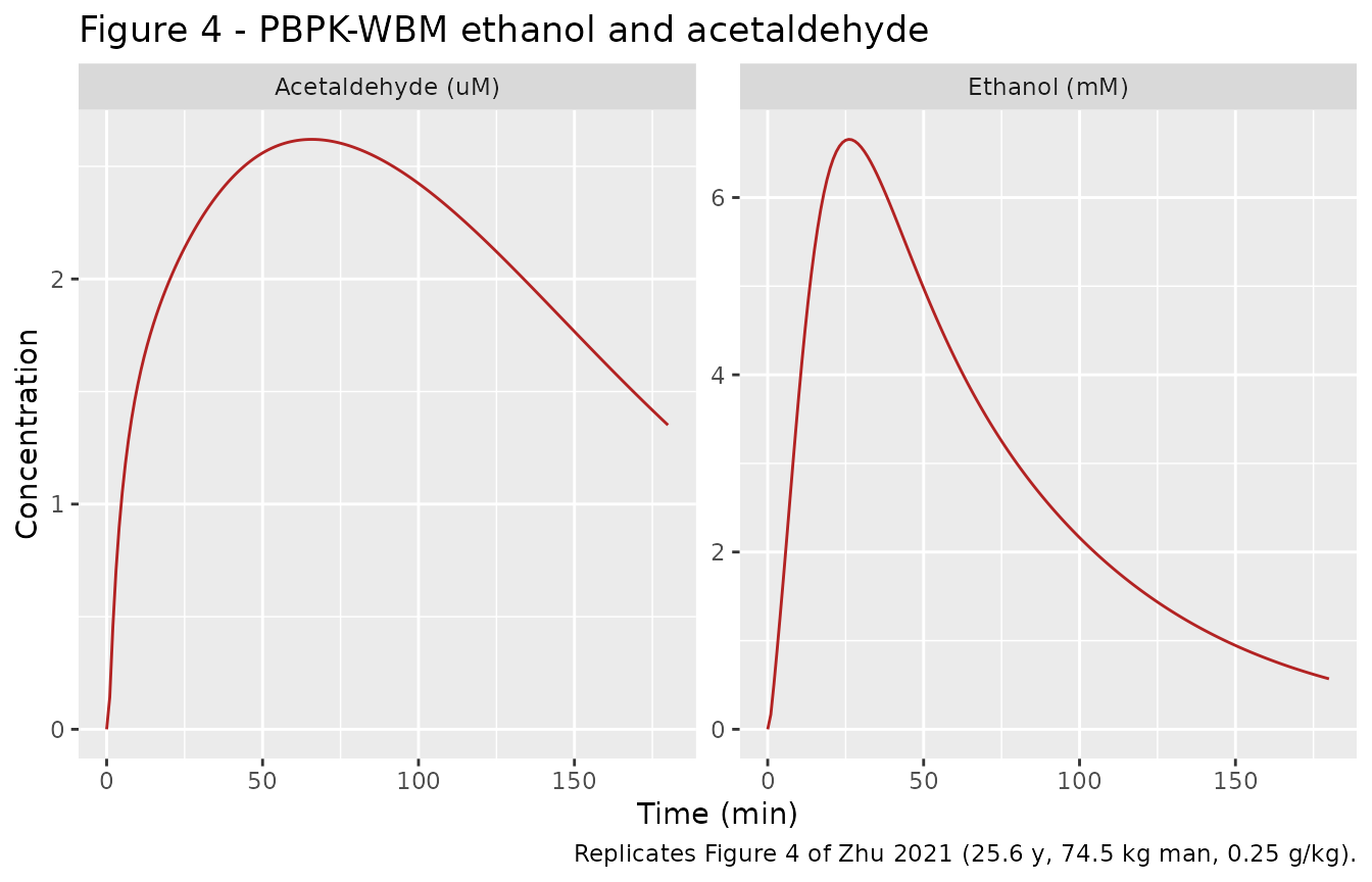
The paper reports (Results, “Predicting acetaldehyde exposure”) model
AUCs of 526.14 mMmin (ethanol) and 377.72 uMmin (acetaldehyde)
over the observation window, against experimental Jones AUCs of 538.5
and 353.25. The authors’ deposited PBPK-WBM trajectory over 0-180 min
integrates to 517.2 mMmin and 373.4 uMmin. This vignette’s
lsoda solve reproduces the deposited trajectory:
etoh_auc <- auc(s4$time, s4$Cc)
acald_auc <- auc(s4$time, s4$Cc_acald * 1000)
etoh_cmax <- cmax(s4$Cc)
acald_cmax <- cmax(s4$Cc_acald * 1000)

fig4_tab <- tibble::tibble(
  Quantity = c("Ethanol AUC0-180 (mM*min)", "Ethanol Cmax (mM)",
               "Acetaldehyde AUC0-180 (uM*min)", "Acetaldehyde Cmax (uM)"),
  Simulated = round(c(etoh_auc, etoh_cmax, acald_auc, acald_cmax), 2),
  Deposited = c(517.2, 6.68, 373.4, 2.60),
  Paper = c(526.14, NA, 377.72, NA)
)
knitr::kable(fig4_tab, caption = "Figure 4 exposure vs the deposited trajectory.")| Quantity | Simulated | Deposited | Paper |
|---|---|---|---|
| Ethanol AUC0-180 (mM*min) | 516.61 | 517.20 | 526.14 |
| Ethanol Cmax (mM) | 6.66 | 6.68 | NA |
| Acetaldehyde AUC0-180 (uM*min) | 377.85 | 373.40 | 377.72 |
| Acetaldehyde Cmax (uM) | 2.62 | 2.60 | NA |
# Deterministic solve: bound is the lsoda-vs-Euler integrator gap (a few %),
# tight enough to catch a mis-transcribed constant (which moves these by tens
# of percent).
stopifnot(
  abs(etoh_auc / 517.2 - 1) < 0.05,
  abs(acald_auc / 373.4 - 1) < 0.06,
  abs(etoh_cmax / 6.68 - 1) < 0.05,
  abs(acald_cmax / 2.60 - 1) < 0.08
)
PKNCA validation - ethanol single drink
Ethanol elimination is zero-order over most of the profile (hepatic
ADH is saturated well above its Km of 1 mmol/L), so a
terminal half-life and AUCinf are not meaningful for this
drug. Cmax, Tmax and AUClast are,
and they are what the paper reports. The PKNCA table below computes them
for the Figure 4 single-drink ethanol profile and compares against the
deposited trajectory and the paper’s reported model AUC.
nca_conc <- s4 |>
  dplyr::filter(!is.na(Cc)) |>
  dplyr::transmute(id = 1L, time, conc = Cc, scenario = "0.25 g/kg drink")

# The solve grid already starts at time 0 (Cc = 0 pre-absorption); guarantee it.
nca_conc <- dplyr::bind_rows(
  nca_conc,
  nca_conc |> dplyr::distinct(id, scenario) |> dplyr::mutate(time = 0, conc = 0)
) |>
  dplyr::distinct(id, scenario, time, .keep_all = TRUE) |>
  dplyr::arrange(id, time)

conc_obj <- PKNCA::PKNCAconc(nca_conc, conc ~ time | scenario + id)
dose_obj <- PKNCA::PKNCAdose(
  data.frame(id = 1L, scenario = "0.25 g/kg drink", time = 0,
             amt = 0.25 * ref_cov$WT / MW_ETOH * 1000),
  amt ~ time | scenario + id
)
nca_res <- PKNCA::pk.nca(PKNCA::PKNCAdata(
  conc_obj, dose_obj,
  intervals = data.frame(start = 0, end = 180,
                         cmax = TRUE, tmax = TRUE, auclast = TRUE)
))

published <- tibble::tibble(
  scenario = "0.25 g/kg drink",
  cmax = 6.68, # deposited PBPK-WBM trajectory (Fig 4)
  tmax = 26.1, # deposited PBPK-WBM trajectory (Fig 4)
  auclast = 526.14 # paper Results text (model ethanol AUC)
)

cmp <- nlmixr2lib::ncaComparisonTable(
  simulated = nca_res,
  reference = published,
  by = "scenario",
  units = c(cmax = "mmol/L", tmax = "min", auclast = "mmol/L*min"),
  tolerance_pct = 20
)
knitr::kable(cmp,
  caption = paste("Simulated vs reference ethanol NCA (Fig 4 single drink).",
"* differs from reference by more than 20%."))| NCA parameter | scenario | Reference | Simulated | % diff |
|---|---|---|---|---|
| Cmax (mmol/L) | 0.25 g/kg drink | 6.68 | 6.66 | -0.4% |
| Tmax (min) | 0.25 g/kg drink | 26.1 | 26 | -0.4% |
| AUClast (mmol/L*min) | 0.25 g/kg drink | 526 | 517 | -1.8% |
Figure 6 - ALDH2 isoform effect on acetaldehyde
Acetaldehyde is cleared almost entirely by hepatic ALDH2. The
isoform-activity column of Table 4 scales f_aldh2. The
paper (Results, “Impact of ALDH isoform”) states the East-Asian ALDH2.2
isoform gives “a 17-fold increase in exposure in the first 500 minutes
when compared to the wildtype”.
Although the paper labels Figs 6-8 as PBPK-WBM output, the curves
saved in the authors’ deposited figure files are reproduced exactly (to
the plotted precision) by the base PBPK with the genome-scale excretion
fractions switched off, and not by the coupled model. Figs 6-8 below are
therefore simulated with wbm = FALSE, and compared against
the Cmax, Tmax and AUC0-500 read from those deposited figure files. The
remaining differences come from integrating with lsoda
rather than the authors’ 0.1-min explicit Euler step.
isoforms <- tibble::tribble(
  ~isoform,          ~activity,
  "ALDH2.1 - WT",     1.000,
  "ALDH2.2 - E504K",  0.015,
  "ALDH2.3 - I41V",   0.600,
  "ALDH2.4 - P92T",   0.325,
  "ALDH2.5 - T244M",  0.360,
  "ALDH2.6 - V304M",  0.125,
  "ALDH2.7 - R338W",  0.230
)

fig6 <- lapply(seq_len(nrow(isoforms)), function(i) {
  s <- solve_scen(drink = 0.20, tmax = 500,
                  params = c(f_aldh2 = isoforms$activity[i]), wbm = FALSE)
  data.frame(isoform = isoforms$isoform[i], time = s$time,
             acald = s$Cc_acald * 1000)
}) |> bind_rows()

ggplot(fig6, aes(time, acald, colour = isoform)) +
  geom_line() +
  labs(x = "Time (min)", y = "Acetaldehyde (uM)",
       title = "Figure 6a - ALDH2 isoform effect on acetaldehyde",
       caption = "Replicates Figure 6a of Zhu 2021.")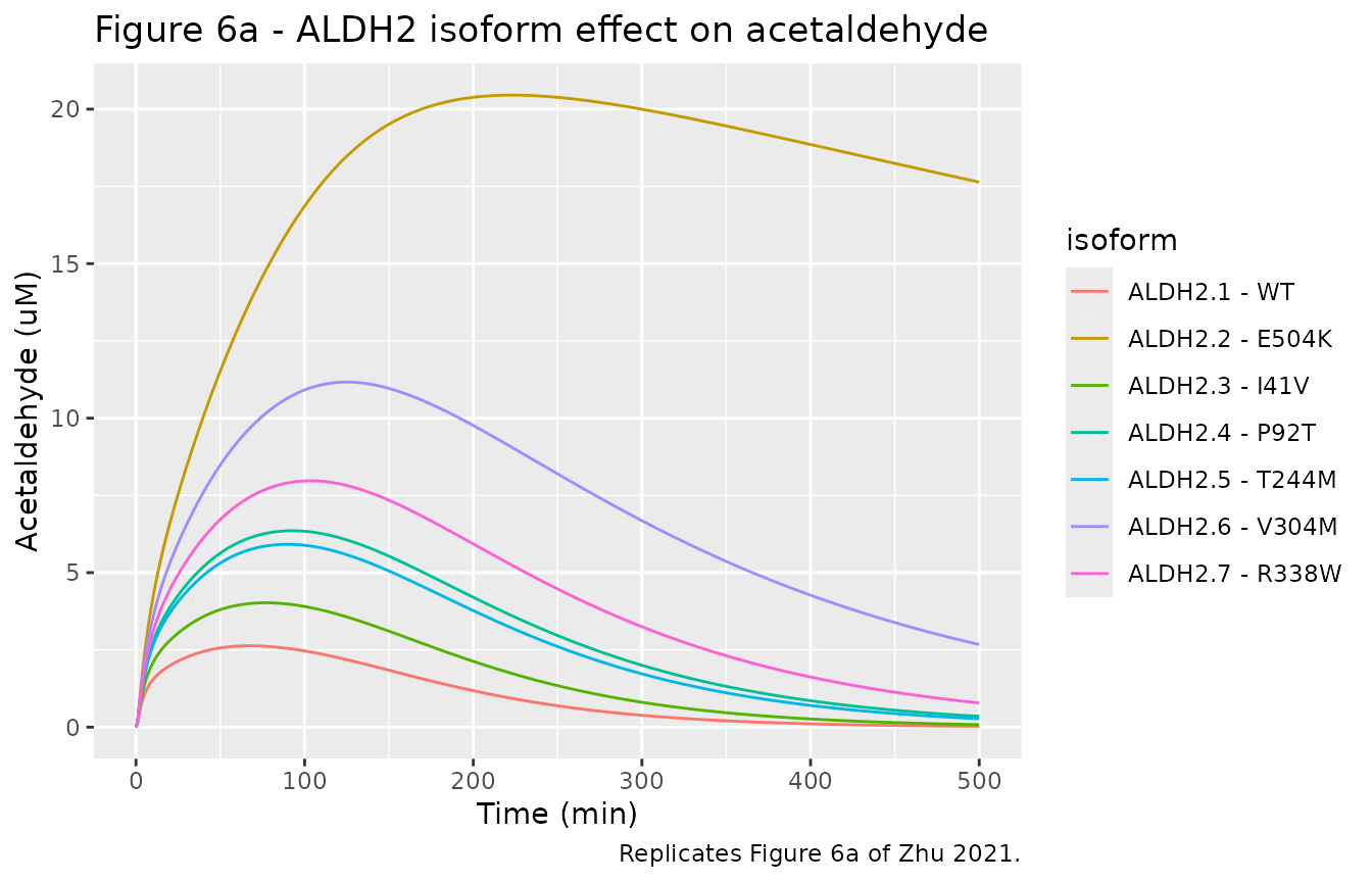
fig6_auc <- fig6 |>
  group_by(isoform) |>
  summarise(auc0_500 = auc(time, acald), .groups = "drop")
wt_auc <- fig6_auc$auc0_500[fig6_auc$isoform == "ALDH2.1 - WT"]
fig6_auc$fold_vs_wt <- round(fig6_auc$auc0_500 / wt_auc, 2)
knitr::kable(fig6_auc, digits = 1,
caption = "Acetaldehyde AUC0-500 by ALDH2 isoform.")| isoform | auc0_500 | fold_vs_wt |
|---|---|---|
| ALDH2.1 - WT | 510.7 | 1.0 |
| ALDH2.2 - E504K | 8797.6 | 17.2 |
| ALDH2.3 - I41V | 848.2 | 1.7 |
| ALDH2.4 - P92T | 1541.6 | 3.0 |
| ALDH2.5 - T244M | 1397.7 | 2.7 |
| ALDH2.6 - V304M | 3550.1 | 7.0 |
| ALDH2.7 - R338W | 2127.8 | 4.2 |
# ALDH2.2 acetaldehyde AUC0-500 is ~17x wild type (paper's headline claim).
ald22_fold <- fig6_auc$fold_vs_wt[fig6_auc$isoform == "ALDH2.2 - E504K"]
stopifnot(ald22_fold > 15, ald22_fold < 19)
# Every reduced-activity isoform raises acetaldehyde exposure over WT.
stopifnot(all(fig6_auc$fold_vs_wt[fig6_auc$isoform != "ALDH2.1 - WT"] > 1))
PKNCA validation against the deposited Figure 6 curves
# One deterministic profile per isoform. The grid starts at time 0, so every
# profile carries the pre-dose zero PKNCA needs to anchor AUC0-500.
nca6_conc <- fig6 |>
  dplyr::filter(!is.na(acald)) |>
  dplyr::transmute(id = 1L, isoform, time, Cc = acald)
nca6_dose <- isoforms |>
  dplyr::transmute(id = 1L, isoform, time = 0,
                   amt = 0.25 * ref_cov$WT / MW_ETOH * 1000)

nca6 <- PKNCA::pk.nca(PKNCA::PKNCAdata(
  PKNCA::PKNCAconc(nca6_conc, Cc ~ time | isoform + id),
  PKNCA::PKNCAdose(nca6_dose, amt ~ time | isoform + id),
  intervals = data.frame(start = 0, end = 500, cmax = TRUE, tmax = TRUE,
                         auclast = TRUE)
))

# Cmax (uM), Tmax (min) and AUC0-500 (uM*min) of each acetaldehyde curve in
# the authors' deposited figure file ALDH/'ALDH2 Polymorphisms.fig'.
deposited6 <- tibble::tribble(
  ~isoform,           ~cmax,   ~tmax, ~auclast,
  "ALDH2.1 - WT",      2.633,   67.4,    510.7,
  "ALDH2.2 - E504K",  20.455,  223.2,   8797.2,
  "ALDH2.3 - I41V",    4.025,   77.0,    848.2,
  "ALDH2.4 - P92T",    6.356,   92.8,   1541.6,
  "ALDH2.5 - T244M",   5.917,   89.9,   1397.7,
  "ALDH2.6 - V304M",  11.169,  125.1,   3550.3,
  "ALDH2.7 - R338W",   7.974,  103.6,   2127.8
)

cmp6 <- nlmixr2lib::ncaComparisonTable(
  simulated = nca6,
  reference = deposited6,
  by = "isoform",
  units = c(cmax = "uM", tmax = "min", auclast = "uM*min"),
  tolerance_pct = 20
)
knitr::kable(cmp6,
  caption = paste("Simulated vs deposited Figure 6 acetaldehyde NCA by ALDH2",
"isoform. * differs from reference by more than 20%."))| NCA parameter | isoform | Reference | Simulated | % diff |
|---|---|---|---|---|
| Cmax (uM) | ALDH2.1 - WT | 2.63 | 2.63 | +0.0% |
| Cmax (uM) | ALDH2.2 - E504K | 20.5 | 20.5 | -0.0% |
| Cmax (uM) | ALDH2.3 - I41V | 4.03 | 4.02 | -0.0% |
| Cmax (uM) | ALDH2.4 - P92T | 6.36 | 6.36 | +0.0% |
| Cmax (uM) | ALDH2.5 - T244M | 5.92 | 5.92 | +0.0% |
| Cmax (uM) | ALDH2.6 - V304M | 11.2 | 11.2 | -0.0% |
| Cmax (uM) | ALDH2.7 - R338W | 7.97 | 7.97 | -0.0% |
| Tmax (min) | ALDH2.1 - WT | 67.4 | 67 | -0.6% |
| Tmax (min) | ALDH2.2 - E504K | 223 | 223 | -0.1% |
| Tmax (min) | ALDH2.3 - I41V | 77 | 77 | +0.0% |
| Tmax (min) | ALDH2.4 - P92T | 92.8 | 93 | +0.2% |
| Tmax (min) | ALDH2.5 - T244M | 89.9 | 90 | +0.1% |
| Tmax (min) | ALDH2.6 - V304M | 125 | 125 | -0.1% |
| Tmax (min) | ALDH2.7 - R338W | 104 | 103 | -0.6% |
| AUClast (uM*min) | ALDH2.1 - WT | 511 | 511 | -0.0% |
| AUClast (uM*min) | ALDH2.2 - E504K | 8800 | 8800 | +0.0% |
| AUClast (uM*min) | ALDH2.3 - I41V | 848 | 848 | +0.0% |
| AUClast (uM*min) | ALDH2.4 - P92T | 1540 | 1540 | -0.0% |
| AUClast (uM*min) | ALDH2.5 - T244M | 1400 | 1400 | +0.0% |
| AUClast (uM*min) | ALDH2.6 - V304M | 3550 | 3550 | -0.0% |
| AUClast (uM*min) | ALDH2.7 - R338W | 2130 | 2130 | -0.0% |
Figure 7 - disulfiram effect on acetaldehyde
A steady blood disulfiram level inhibits ALDH2 through the S3 Text quadratic. The paper simulates 0, 2, 4, 6 and 8 mg/L.
dsf_levels <- c(0, 2, 4, 6, 8)
fig7 <- lapply(dsf_levels, function(d) {
  s <- solve_scen(drink = 0.20, tmax = 500,
                  params = c(c_disulfiram = d), wbm = FALSE)
  data.frame(disulfiram = paste0(d, " mg/L"), time = s$time,
             acald = s$Cc_acald * 1000)
}) |> bind_rows()

ggplot(fig7, aes(time, acald, colour = disulfiram)) +
  geom_line() +
  labs(x = "Time (min)", y = "Acetaldehyde (uM)",
       title = "Figure 7a - disulfiram effect on acetaldehyde",
       caption = "Replicates Figure 7a of Zhu 2021.")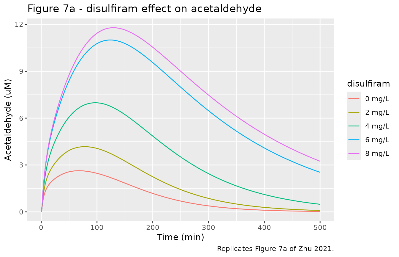
fig7_auc <- fig7 |>
  group_by(disulfiram) |>
  summarise(auc0_500 = auc(time, acald), .groups = "drop") |>
  mutate(order = as.numeric(sub(" mg/L", "", disulfiram))) |>
  arrange(order)
knitr::kable(fig7_auc[, c("disulfiram", "auc0_500")], digits = 1,
caption = "Acetaldehyde AUC0-500 by blood disulfiram level.")| disulfiram | auc0_500 |
|---|---|
| 0 mg/L | 510.7 |
| 2 mg/L | 887.4 |
| 4 mg/L | 1758.1 |
| 6 mg/L | 3466.7 |
| 8 mg/L | 3862.9 |
Figure 8 - repeated drinking
A drink every 60 min (14 g standard drinks at 60, 120 and 180 min on top of the 0.25 g/kg starting drink). Acetaldehyde keeps accumulating while ethanol is still present.
s8 <- solve_scen(gkg = 0.25, drink = 0.20, tmax = 500,
                 extra_g = c("60" = 14, "120" = 14, "180" = 14), wbm = FALSE)

bind_rows(
  data.frame(time = s8$time, analyte = "Ethanol (mM)", conc = s8$Cc),
  data.frame(time = s8$time, analyte = "Acetaldehyde (uM)", conc = s8$Cc_acald * 1000)
) |>
  ggplot(aes(time, conc)) +
  geom_line(colour = "#1f5c99") +
  facet_wrap(~analyte, scales = "free_y") +
  labs(x = "Time (min)", y = "Concentration",
       title = "Figure 8 - repeated drinking (q60 min)",
       caption = "Replicates Figure 8a,b of Zhu 2021.")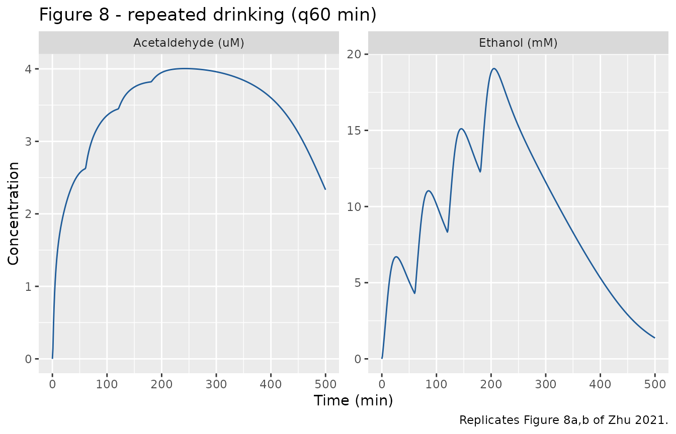
Enzyme expression (Figure 5)
Reducing hepatic enzyme expression (fexpr_liver) raises
ethanol exposure and lowers acetaldehyde exposure, matching the clinical
trend the paper cites (Wicht et al.).
expr_levels <- c(1, 0.75, 0.5, 0.25, 0.1)
fig5 <- lapply(expr_levels, function(f) {
  s <- solve_scen(drink = 0.20, tmax = 180,
                  params = c(fexpr_liver = f), wbm = TRUE)
  data.frame(expr = f, etoh_auc = auc(s$time, s$Cc),
             acald_auc = auc(s$time, s$Cc_acald * 1000))
}) |> bind_rows()
knitr::kable(fig5, digits = 1,
caption = "Ethanol and acetaldehyde AUC0-180 by hepatic enzyme expression.")| expr | etoh_auc | acald_auc |
|---|---|---|
| 1.0 | 516.6 | 377.8 |
| 0.8 | 831.5 | 345.9 |
| 0.5 | 1171.1 | 231.6 |
| 0.2 | 1399.8 | 95.6 |
| 0.1 | 1465.9 | 23.7 |
Assumptions and deviations
-
Genome-scale layer reduced to its continuous limit.
The published model couples the PBPK to the Harvey whole-body
genome-scale reconstruction by dynamic flux-balance analysis, re-solving
a linear programme whenever the Michaelis-Menten rate drifts more than a
set tolerance from the current flux. The linear programme, its 81,094
reactions and the CPLEX solver are not reproducible in rxode2, and the
deposited S1/S2 Tables list the ethanol- and acetaldehyde-related
reactions by name only, without flux values. In the authors’ deposited
runs the solver holds urine and sweat excretion at their 10% upper
bounds and breath at its fixed 0.5%, so the continuous limit is the ODE
system encoded here with those excretions entered as fixed fractions of
the hepatic ADH rate (
f_urine_wbm,f_sweat_wbm,f_breath_wbm). Setting them to zero recovers the base PBPK (ModelVer 1) that generated Figs 6-8. This model is therefore the paper’s ODE model, not its flux-balance optimiser; it reproduces the paper’s simulated trajectories but cannot re-derive the flux bounds from the genome-scale network. -
kSI sign typo. S2 Text Eq S2.3 prints
kSI = -0.006*Drink%^2 - 0.0686*Drink% + 0.0615, but the depositedmain.muses+0.0686. The+sign reproduces the authors’ deposited small-intestine-lumen trajectory exactly, so the model uses+0.0686and treats the printed-as a typographical error. -
Figure 3 used a preliminary parameterisation. The
gut-absorption fitting figure (Fig 3, Mitchell 82.66 kg subject) was
generated with a hepatic ADH
Vmaxof 1.5 mM/min (stated in its caption) and a different absorbed fraction, before the model adopted the UmulisVmax = 2.2used for every later figure. The packaged model ships the finalVmax = 2.2; it does not reproduce Fig 3 at its defaults. Figs 4-8, which use the final parameterisation, are reproduced above. - Deterministic. No between-subject variability or residual error was reported or encoded. The model returns typical-value trajectories.
- Men only. The organ correlations and the deposited driver support male physiology only.
-
Dosing units. Ethanol enters the
stomachstate in mmol withf(stomach) = 0.8(the authors’ 80% assumed bioavailability into the gastric lumen). Convert ag/kgdrink with the subject’s weight and 46.0684 g/mol before building the event table, as the helper above does. -
Non-paper provenance. All structural constants come
from the paper text, its supplements (S1-S3 Text), or the authors’
deposited MATLAB code (
github.com/LMSE/HH-PBPK-Ethanol, commitb14305a), which reproduces Figs 4-8. The ALDH2 isoform activities (Table 4) trace to Chan et al. 2020 viaaALDHtype.m; the disulfiram correlation (S3 Text) to Kitson 1978 sheep liver data.