Radiation + radiosensitizer tumor model (Cardilin 2018)
Source:vignettes/articles/Cardilin_2018_radiation_radiosensitizer_mouse.Rmd
Cardilin_2018_radiation_radiosensitizer_mouse.RmdModel and source
- Citation: Cardilin T, Almquist J, Jirstrand M, Zimmermann A, El Bawab S, Gabrielsson J. Model-Based Evaluation of Radiation and Radiosensitizing Agents in Oncology. CPT Pharmacometrics Syst Pharmacol. 2018;7(1):51-58. doi:10.1002/psp4.12268. PMID 29218836; PMCID PMC5784742.
- Description: Preclinical (mouse, FaDu head-and-neck xenograft). Tumor growth inhibition model for combination therapy with ionizing radiation and a radiosensitizer (linear-quadratic radiation kill with a damage-compartment transit chain, driven by a one-compartment radiosensitizer PK).
- Article (open access): https://doi.org/10.1002/psp4.12268
- Supplement (Europe PMC, PMC5784742): https://www.ebi.ac.uk/europepmc/webservices/rest/PMC5784742/supplementaryFiles
This is a preclinical tumor-growth-inhibition (TGI) model for combination therapy with ionizing radiation and a radiosensitizing compound (anonymized “RS1” in the source), fit to FaDu head-and-neck xenograft data in mice. The proliferating compartment grows logistically and feeds a three-stage natural-death transit chain. Radiation acts through the linear-quadratic (LQ) surviving-fraction theory as a near-instantaneous transfer of proliferating cells into an irradiated chain (which is allowed at most one further division before dying). The radiosensitizer’s one-compartment plasma PK drives both a small enhancement of natural cell death and a strong synergistic enhancement of the radiation kill.
Population
The structural model was estimated from a FaDu (human head-and-neck squamous-cell-carcinoma) xenograft experiment in female CD1 nu/nu or NMRI nu/nu mice (Supplementary Material B of the source). The primary tumor dataset comprised 80 mice in eight groups of ten: (A) vehicle, (B) radiation 2 Gy, (C-E) RS1 monotherapy 10/50/200 mg/kg, and (F-H) combination of 2 Gy + RS1 10/50/200 mg/kg, dosed once daily on days 3-7. RS1 was given orally 10 minutes before each irradiation. A second 10-mouse dataset (2 Gy + RS1 25 mg/kg, five days per week for six weeks) was used for prediction (Figure 5 of the source). The radiosensitizer PK was estimated separately from 147 tumor-bearing female mice across five single-dose studies (Supplementary Table SI). Between-subject variability was estimated for the initial tumor volume, the tumor capacity, and the two PK parameters.
The same information is available programmatically via
readModelDb("Cardilin_2018_radiation_radiosensitizer_mouse")$population.
Source trace
Per-parameter origins are recorded as in-file comments next to each
ini() entry. The table collects them for review.
| Equation / parameter | Value | Source location |
|---|---|---|
lkg (growth rate kg) |
0.50 1/day | Table 1 |
lkk (kill rate kk) |
0.28 1/day | Table 1 |
lcap (capacity K) |
2200 mm^3 | Table 1 |
lv0 (initial volume V0) |
40.0 mm^3 | Table 1 |
lalpha (LQ alpha) |
0.08 1/Gy | Table 1 |
abratio (alpha/beta, fixed) |
10 Gy | Methods + Table 1 footnote |
laDeath (natural-death stim., paper “a”) |
0.09 mL/ug | Table 1 + Discussion (“9% per ug/mL”) |
lbRad (radiation synergy, paper “b”) |
0.45 mL/ug | Table 1 + Discussion (“45% per ug/mL”) |
lke (RS1 elimination) |
0.21 1/h (x 24 = 5.04 1/day) | Supplementary Table SI |
lvf (RS1 apparent V/F) |
9.51 L/kg | Supplementary Table SI |
radDose (per fraction) |
2 Gy | Methods |
etalv0 / etalcap
|
BSV 21% / 32% | Table 1 |
etalvf / etalke
|
BSV 88% / 15% | Supplementary Table SI |
propSd |
23% | Table 1 (sigma) |
| ODE system (Eq. 6), ICs (Eq. 7) | n/a | Methods + Mathematica supplement (s008) |
PK solution C(t)=D F / V exp(-ke t)
|
n/a | Supplementary Material A, Eq. 18 |
Simulation set-up
Radiation is delivered as a unit bolus (amt = 1) into
the radDepot compartment at each irradiation time; the
per-fraction radiation dose (Gy) is the model parameter
radDose (default 2). RS1 is dosed (mg/kg) into the
central compartment. The observation tumor_vol
is the total tumor volume (sum of all six tumor compartments, mm^3).
mod <- readModelDb("Cardilin_2018_radiation_radiosensitizer_mouse")
#> ℹ Radiation is given as a unit bolus (amt=1) into the radDepot compartment at each irradiation time; the per-fraction radiation dose (Gy) is the parameter radDose (default 2). RS1 is dosed (mg/kg) into the central compartment. Observation tumor_vol is total tumor volume (mm^3).
mod_typ <- rxode2::zeroRe(mod)   # typical-value (no between-subject variability)
#> ℹ parameter labels from comments will be replaced by 'label()'

# Build an event table for one treatment group on the days-3-7 schedule.
make_group <- function(rs_dose = 0, irradiate = FALSE, days = 3:7,
                       tmax = 30, by = 0.25) {
  ev <- rxode2::et(seq(0, tmax, by = by))
  if (rs_dose > 0)
    for (d in days) ev <- rxode2::et(ev, amt = rs_dose, cmt = "central",
                                     time = d - 10/1440)  # 10 min before IR
  if (irradiate)
    for (d in days) ev <- rxode2::et(ev, amt = 1, cmt = "radDepot", time = d)
  ev
}
Replicate Figure 2 – tumor volume by treatment group
groups <- list(
  "A: vehicle"            = make_group(0,   FALSE),
  "B: radiation 2 Gy"     = make_group(0,   TRUE),
  "E: RS1 200 mg/kg"      = make_group(200, FALSE),
  "F: 2 Gy + RS1 10"      = make_group(10,  TRUE),
  "G: 2 Gy + RS1 50"      = make_group(50,  TRUE),
  "H: 2 Gy + RS1 200"     = make_group(200, TRUE)
)
traj <- bind_rows(lapply(names(groups), function(g) {
  s <- as.data.frame(rxode2::rxSolve(mod_typ, groups[[g]]))
  data.frame(time = s$time, tumor_vol = s$tumor_vol, group = g)
}))
#> ℹ omega/sigma items treated as zero: 'etalv0', 'etalcap', 'etalvf', 'etalke'
#> ℹ omega/sigma items treated as zero: 'etalv0', 'etalcap', 'etalvf', 'etalke'
#> ℹ omega/sigma items treated as zero: 'etalv0', 'etalcap', 'etalvf', 'etalke'
#> ℹ omega/sigma items treated as zero: 'etalv0', 'etalcap', 'etalvf', 'etalke'
#> ℹ omega/sigma items treated as zero: 'etalv0', 'etalcap', 'etalvf', 'etalke'
#> ℹ omega/sigma items treated as zero: 'etalv0', 'etalcap', 'etalvf', 'etalke'

ggplot(traj, aes(time, tumor_vol)) +
  geom_line(linewidth = 0.7) +
  facet_wrap(~group) +
  labs(x = "Time (day)", y = expression("Tumor volume (mm"^3*")"),
       title = "Replicates Figure 2 of Cardilin et al. (2018)",
       caption = "Typical-value tumor growth; radiation 2 Gy/dose on days 3-7.") +
  theme_bw()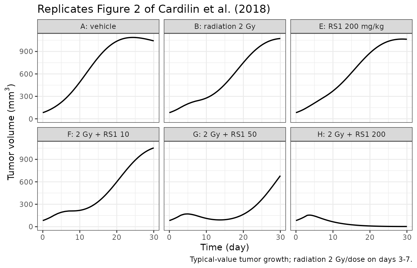
Vehicle (A) grows approximately exponentially toward the capacity; RS1 monotherapy (E) deviates only slightly from vehicle; radiation alone (B) slows growth considerably but does not produce regression; and combination therapy shrinks the tumor in a dose-dependent way, with the highest dose (H) driving rapid, near-complete eradication. This matches the source narrative and Figure 2.
Quantitative validation – per-fraction kill fractions
The source reports that a single 2 Gy fraction kills 17% of proliferating cells, rising to 24%, 46%, and 85% in combination with RS1 10, 50, and 200 mg/kg (Discussion). We reproduce these by measuring the drop in the cycling-cells compartment across one fraction.
kill_one <- function(rs_dose) {
  ev <- rxode2::et(seq(0, 4, by = 0.001))
  if (rs_dose > 0) ev <- rxode2::et(ev, amt = rs_dose, cmt = "central",
                                    time = 3 - 10/1440)
  ev <- rxode2::et(ev, amt = 1, cmt = "radDepot", time = 3)
  s <- as.data.frame(rxode2::rxSolve(mod_typ, ev, maxsteps = 1e6,
                                     atol = 1e-9, rtol = 1e-9))
  pre  <- s$cycling_cells[which.min(abs(s$time - 2.99))]
  post <- s$cycling_cells[which.min(abs(s$time - 3.05))]  # after the fast kill spike
  100 * (1 - post / pre)
}
kill_tab <- data.frame(
  scenario  = c("2 Gy alone", "2 Gy + RS1 10", "2 Gy + RS1 50", "2 Gy + RS1 200"),
  simulated = round(sapply(c(0, 10, 50, 200), kill_one), 0),
  published = c(17, 24, 46, 85)
)
#> ℹ omega/sigma items treated as zero: 'etalv0', 'etalcap', 'etalvf', 'etalke'
#> ℹ omega/sigma items treated as zero: 'etalv0', 'etalcap', 'etalvf', 'etalke'
#> ℹ omega/sigma items treated as zero: 'etalv0', 'etalcap', 'etalvf', 'etalke'
#> ℹ omega/sigma items treated as zero: 'etalv0', 'etalcap', 'etalvf', 'etalke'
kill_tab |>
  dplyr::rename(
    "Scenario"           = scenario,
    "Simulated kill (%)" = simulated,
    "Published kill (%)" = published
  ) |>
knitr::kable(caption = "Per-fraction proliferating-cell kill: model vs source.")| Scenario | Simulated kill (%) | Published kill (%) |
|---|---|---|
| 2 Gy alone | 17 | 17 |
| 2 Gy + RS1 10 | 24 | 24 |
| 2 Gy + RS1 50 | 46 | 46 |
| 2 Gy + RS1 200 | 86 | 85 |
The combination kill fractions reproduce the published values; the 2 Gy-alone value reads slightly low because it is measured shortly after the kill, during which the surviving cells simultaneously grow and die.
Quantitative validation – RS1 average plasma concentrations
The source reports average daily RS1 plasma concentrations of 0.52, 0.9, and 8.2 ug/mL for 25, 48, and 400 mg/kg (main text and Supplementary Material D). We reproduce these from the one-compartment PK by averaging concentration over a one-day dosing interval.
cavg <- function(dose) {
  ev <- rxode2::et(amt = dose, cmt = "central", time = 0) |>
    rxode2::et(seq(0, 1, by = 0.001))
  s <- as.data.frame(rxode2::rxSolve(mod_typ, ev))
  # trapezoidal mean over [0, 1] day
  mean(0.5 * (head(s$Cc, -1) + tail(s$Cc, -1)))
}
conc_tab <- data.frame(
  dose_mgkg = c(25, 48, 400),
  simulated = round(sapply(c(25, 48, 400), cavg), 2),
  published = c(0.52, 0.9, 8.2)
)
#> ℹ omega/sigma items treated as zero: 'etalv0', 'etalcap', 'etalvf', 'etalke'
#> ℹ omega/sigma items treated as zero: 'etalv0', 'etalcap', 'etalvf', 'etalke'
#> ℹ omega/sigma items treated as zero: 'etalv0', 'etalcap', 'etalvf', 'etalke'
conc_tab |>
  dplyr::rename(
    "RS1 dose (mg/kg)"            = dose_mgkg,
    "Simulated mean conc (ug/mL)" = simulated,
    "Published mean conc (ug/mL)" = published
  ) |>
knitr::kable(caption = "Average daily RS1 plasma concentration: model vs source.")| RS1 dose (mg/kg) | Simulated mean conc (ug/mL) | Published mean conc (ug/mL) |
|---|---|---|
| 25 | 0.52 | 0.52 |
| 48 | 0.99 | 0.90 |
| 400 | 8.29 | 8.20 |
Replicate Figure 5 – six-week combination prediction
The second (prediction) dataset used 2 Gy + RS1 25 mg/kg five days per week (Mon-Fri) for six weeks. We simulate the population (5th/50th/95th percentiles) on this schedule.
treat_days <- as.vector(outer(1:5, 7 * (0:5), `+`))  # Mon-Fri for 6 weeks
treat_days <- sort(treat_days)

ev6 <- rxode2::et(seq(0, 45, by = 0.5))
for (d in treat_days) {
  ev6 <- rxode2::et(ev6, amt = 25, cmt = "central", time = d - 10/1440)
  ev6 <- rxode2::et(ev6, amt = 1,  cmt = "radDepot", time = d)
}

sim6 <- rxode2::rxSolve(mod, ev6, nSub = 200, maxsteps = 1e6) |>
  as.data.frame()
#> ℹ parameter labels from comments will be replaced by 'label()'

vpc6 <- sim6 |>
  group_by(time) |>
  summarise(Q05 = quantile(tumor_vol, 0.05, na.rm = TRUE),
            Q50 = quantile(tumor_vol, 0.50, na.rm = TRUE),
            Q95 = quantile(tumor_vol, 0.95, na.rm = TRUE), .groups = "drop")

ggplot(vpc6, aes(time, Q50)) +
  geom_ribbon(aes(ymin = Q05, ymax = Q95), alpha = 0.25) +
  geom_line(linewidth = 0.7) +
  labs(x = "Time (day)", y = expression("Tumor volume (mm"^3*")"),
       title = "Replicates Figure 5 of Cardilin et al. (2018)",
       caption = "2 Gy + RS1 25 mg/kg, Mon-Fri for 6 weeks; 200 virtual mice.") +
  theme_bw()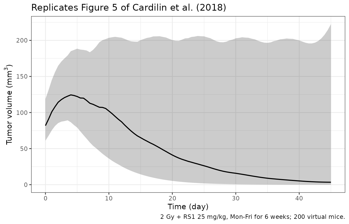
Consistent with Figure 5 and the source narrative, the clinically relevant six-week schedule drives the tumor into sustained regression (most simulated animals are eradicated by the end of treatment).
Dimensional analysis
The model mixes day-based rates, mm^3 volumes, ug/mL concentrations,
and Gy radiation doses. Each ODE term is dimensionally consistent with
d/dt(state) = volume/time = mm^3/day:
| Term | Units | Notes |
|---|---|---|
kg * cycling_cells * logi |
(1/day)(mm^3)(-) = mm^3/day |
logi dimensionless |
(1 + aDeath*Cc) * kk * cycling_cells |
(-)(1/day)(mm^3) = mm^3/day |
aDeath*Cc = (mL/ug)(ug/mL) dimensionless |
killHaz * cycling_cells |
(1/day)(mm^3) = mm^3/day | see below |
lethal |
(-)(1/Gy * Gy) = dimensionless | LQ lethal lesions, alpha*radDose + beta*radDose^2
|
krad * radDepot |
(1/day)(-) integrates to 1 per fraction | numerical delta-trigger |
Cc = central / vf |
(mg/kg)/(L/kg) = mg/L = ug/mL | RS1 plasma concentration |
ke * central |
(1/day)(mg/kg) = (mg/kg)/day | RS1 elimination |
The radiation kill hazard
killHaz = lethal * krad * radDepot integrates over a
fraction to lethal (since the unit radDepot
bolus has integral 1 under the krad decay), so the
proliferating pool is multiplied by the LQ surviving fraction
exp(-lethal) = exp(-(1 + bRad*Cc)(alpha*D + beta*D^2)).
Assumptions and deviations
-
Metadata correction (year and name). The dispatch
metadata named the model
Cardilin_2017_CPT_Pharmacometrics_amp_Sys(a queue-generation artifact in which the journal name was placed in the drug slot, and the online-first year 2017 was used). The article’s formal citation is CPT Pharmacometrics Syst Pharmacol 2018;7(1):51-58 (published online 14 December 2017); 2018 is the volume/citation year used by PubMed (PMID 29218836) and matches the on-disk source filename. The compound is anonymized as “RS1” in the source, so the descriptive slotradiation_radiosensitizerand the_mousespecies suffix are used. - Coefficient placement (paper “a” vs “b”). Table 1 of the source and the code variables in the Mathematica supplement label the two radiosensitizer coefficients oppositely. The placement here (natural-death stimulation = 0.09 mL/ug, radiation synergy = 0.45 mL/ug) follows the paper’s quantitative text (“9% increase in natural cell death” and “45% increase in fraction killed” per ug/mL) and is confirmed by the published combination kill fractions (24/46/85% for 2 Gy + RS1 10/50/200 mg/kg), reproduced above.
-
RS1 apparent volume units. Supplementary Table SI
prints
V = 0.0095with the label “mL/kg”. On a ng/mL concentration basis this value is 0.009507 (mg/kg)/(ng/mL) = 9.51 L/kg (the printed label is a mis-transcription). This value reproduces the reported average plasma concentrations (above), so 9.51 L/kg is used. -
Radiation as a near-instantaneous transfer. The
source models irradiation as Dirac-delta mass transfers. This is
implemented with a fast-decaying unit trigger (
radDepot, ratekrad = 5001/day, integral 1 per fraction) so the proliferating pool is multiplied by the LQ surviving fraction.kradis a solver convenience, not a fitted parameter; increasing it sharpens the approximation. -
Between-subject variability scale. The source
reports BSV as
sqrt(omega^2) x 100(Table 1 / Table SI footnotes), so log-scale variances are(BSV%/100)^2(V0 0.0441, K 0.1024, V/F 0.7744, ke 0.0225). -
Convention-lint warnings (justified, not errors).
The mechanistic tumor compartments (
cycling_cells,damaged_cells1-3,irrad1-2) and the radiation trigger (radDepot) are not canonical PK compartment names, mirroring the existingoncology_xenograft_simeoni_2004TGI model. The fitted output is total tumor volume (tumor_vol, a non-PK output), whileCcis correctly reserved for the RS1 plasma concentration. The unitsmg/kg(RS1 dose) andug/mL(concentration) are both mass-based and reconcile through the apparent volumeV/F(L/kg); the lint’s prefix-level dimensional check is a false positive. -
Initial total volume. With the Table 1 estimates
the initial total volume is
V0 (1 + (kk/kg) + (kk/kg)^2 + (kk/kg)^3)= 82 mm^3; the source reports ~87 mm^3, the small difference arising from rounding of kg and kk. - Observed data. The original animal-level tumor measurements are not publicly available; the figures above are model simulations on the published dosing schedules.