Fosdagrocorat osteocalcin K-PD (Shoji 2017)
Source:vignettes/articles/Shoji_2017_fosdagrocorat_oc.Rmd
Shoji_2017_fosdagrocorat_oc.RmdModel and source
- Citation: Shoji S, Suzuki A, Conrado DJ, Peterson MC, Hey-Hadavi J, McCabe D, Rojo R, Tammara BK. Dissociated Agonist of Glucocorticoid Receptor or Prednisone for Active Rheumatoid Arthritis: Effects on P1NP and Osteocalcin Pharmacodynamics. CPT Pharmacometrics Syst Pharmacol. 2017;6(7):439-448. doi:10.1002/psp4.12201
- Description: Kinetic-pharmacodynamic (K-PD) model for serum osteocalcin (OC) bone-formation biomarker following once-daily oral fosdagrocorat (PF-04171327, a dissociated agonist of the glucocorticoid receptor) or oral prednisone comparator in adults with rheumatoid arthritis on background methotrexate (Shoji 2017). Sister model to Shoji_2017_fosdagrocorat_p1np: identical K-PD structure (virtual K-PD depot with zero-order Input mg/week and first-order KDE; sigmoid Emax inhibition of biomarker synthesis with Hill coefficient fixed to 1; empirical dose-and-time-dependent rebound multiplier; additive placebo-period slope). For the OC fit Shoji 2017 fixed KDE to the P1NP-derived estimates and fixed Imax to 1 for both drugs, and used independent (not block) IIV on KDE, EDK50, and BL.
- Article: https://doi.org/10.1002/psp4.12201
Population
The osteocalcin (OC) K-PD fit used the same 321-patient phase II
cohort as the sister P1NP analysis (NCT01393639); see Shoji_2017_fosdagrocorat_p1np
for the full demographic summary. For the OC fit Shoji 2017 fixed KDE to
the P1NP-derived estimates (KDE-only re-estimation was unstable for OC
data) and fixed Imax to 1 for both drugs (the unconstrained
OC estimate was close to 1).
Source trace
| Equation / parameter | Value | Source location |
|---|---|---|
lkel (KDE fosdagrocorat) |
fixed(log(0.597)) /week |
Table 2 OC: “KDE Fosdagrocorat FIX” (from P1NP fit) |
dlkel_pred |
fixed(log(0.535/0.597)) |
Table 2 OC: “KDE Prednisone FIX” (from P1NP fit) |
lkd |
log(0.939) /week |
Table 2 OC, “Kd” |
lbl |
log(22.2) ng/mL |
Table 2 OC, “BL” |
imax |
fixed(1) |
Table 2 OC, “Imax FIX” (both drugs) |
ledk50 (EDK50 fos) |
log(148) mg/week |
Table 2 OC, “EDK50 Fosdagrocorat” |
dledk50_pred |
log(122/148) |
Table 2 OC, “EDK50 Prednisone” |
hill |
fixed(1) |
Table 2 OC, “c FIX” |
lrbmax |
log(0.0276) /mg |
Table 2 OC, “RBmax” |
lt50 |
log(2.24) weeks |
Table 2 OC, “T50” |
slp |
0.0675 ng/mL/week |
Table 2 OC, “SLP” |
etalkel |
omega^2 = 1.5129 (123% CV) |
Table 2 OC, “IIV %CV [g_KDE]” |
etaledk50 |
omega^2 = 0.0650 (25.5% CV) |
Table 2 OC, “IIV %CV [g_EDK50]” |
etalbl |
omega^2 = 0.1901 (43.6% CV) |
Table 2 OC, “IIV %CV [g_BL]” |
etaslp |
omega^2 = 0.338^2 = 0.1142 |
Table 2 OC, “IIV SD [g_SLP] = 0.338” |
propSd |
0.141 |
Table 2 OC, “Residual variability %CV [e] = 14.1” |
d/dt(depot_kpd) |
-kel * depot_kpd | Methods, K-PD model equations |
d/dt(effect) |
ks * rebound * inhibition - kd * effect | Methods, K-PD model + Results rebound equation |
OC = effect + slp_i * t |
Observation = response + linear placebo trend | Methods, F(ij) equation |
Virtual cohort
The cohort and dosing scheme mirror the P1NP vignette: 200 virtual subjects per trial arm, 8 weeks active treatment followed by a tapered 4-week period.
set.seed(20170527L)

n_per_arm <- 200L

make_arm <- function(arm_label, dose_qd_mg, drug_pred, n,
                     dose_reduced_mg, id_offset) {
  active_rate  <- 7 * dose_qd_mg
  taper_a_rate <- 3.5  * dose_reduced_mg
  taper_b_rate <- 2.33 * dose_reduced_mg

  ids <- id_offset + seq_len(n)
  dose_ev <- if (dose_qd_mg > 0) {
    bind_rows(
      tibble(id = ids, time = 0,  amt = active_rate * 8,
             rate = active_rate, evid = 1L, cmt = "depot_kpd"),
      tibble(id = ids, time = 8,  amt = taper_a_rate * 2,
             rate = taper_a_rate, evid = 1L, cmt = "depot_kpd"),
      tibble(id = ids, time = 10, amt = taper_b_rate * 2,
             rate = taper_b_rate, evid = 1L, cmt = "depot_kpd")
    )
  } else {
    tibble(id = integer(), time = numeric(), amt = numeric(),
           rate = numeric(), evid = integer(), cmt = character())
  }

  obs_ev <- expand.grid(id = ids,
                        time = c(0, 2, 4, 6, 8, 10, 12, 13)) |>
    as_tibble() |>
    mutate(amt = NA_real_, rate = NA_real_, evid = 0L, cmt = NA_character_)

  bind_rows(dose_ev, obs_ev) |>
    arrange(id, time, desc(evid)) |>
    mutate(arm = arm_label, DOSE = dose_qd_mg, DRUG_PRED = drug_pred)
}

events <- bind_rows(
  make_arm("Placebo",        0,  0, n_per_arm,  0, id_offset =   0L),
  make_arm("Fos 1 mg",       1,  0, n_per_arm,  1, id_offset = 200L),
  make_arm("Fos 5 mg",       5,  0, n_per_arm,  1, id_offset = 400L),
  make_arm("Fos 10 mg",     10,  0, n_per_arm,  1, id_offset = 600L),
  make_arm("Fos 15 mg",     15,  0, n_per_arm,  1, id_offset = 800L),
  make_arm("Pred 5 mg",      5,  1, n_per_arm,  5, id_offset = 1000L),
  make_arm("Pred 10 mg",    10,  1, n_per_arm,  5, id_offset = 1200L)
)

stopifnot(!anyDuplicated(unique(events[, c("id", "time", "evid")])))
Simulation
mod <- readModelDb("Shoji_2017_fosdagrocorat_oc")

sim <- rxode2::rxSolve(
  mod, events = events,
  keep = c("arm", "DOSE", "DRUG_PRED")
) |> as.data.frame()

sim_typ <- rxode2::rxSolve(
  rxode2::zeroRe(mod), events = events,
  keep = c("arm", "DOSE", "DRUG_PRED")
) |> as.data.frame()
#> ℹ omega/sigma items treated as zero: 'etalkel', 'etaledk50', 'etalrbase', 'etaslp'
#> Warning: multi-subject simulation without without 'omega'
Replicate Figure 2 (lower row): VPC of OC percent change from baseline
arm_order <- c("Placebo",
               "Fos 1 mg", "Fos 5 mg", "Fos 10 mg", "Fos 15 mg",
               "Pred 5 mg", "Pred 10 mg")

vpc_summary <- sim |>
  filter(time %in% c(0, 2, 4, 6, 8, 10, 12, 13)) |>
  group_by(arm, id) |>
  mutate(oc_baseline = first(OC[time == 0])) |>
  ungroup() |>
  mutate(cfb_pct = 100 * (OC - oc_baseline) / oc_baseline) |>
  group_by(arm, time) |>
  summarise(
    p10 = quantile(cfb_pct, 0.10, na.rm = TRUE),
    p50 = quantile(cfb_pct, 0.50, na.rm = TRUE),
    p90 = quantile(cfb_pct, 0.90, na.rm = TRUE),
    .groups = "drop"
  ) |>
  mutate(arm = factor(arm, levels = arm_order))

ggplot(vpc_summary, aes(time, p50)) +
  geom_ribbon(aes(ymin = p10, ymax = p90), alpha = 0.25, fill = "darkorange") +
  geom_line(color = "darkorange") +
  geom_hline(yintercept = 0, linetype = "dashed", colour = "grey50") +
  geom_vline(xintercept = 8, linetype = "dotted", colour = "grey50") +
  facet_wrap(~ arm, ncol = 4) +
  labs(x = "Time (weeks)",
       y = "Osteocalcin change from baseline (%)",
       title = "Replicates Figure 2 (bottom row) of Shoji 2017",
       subtitle = "Median (line) and 10-90% predictive interval (shaded) per arm",
       caption = "Vertical dotted line at week 8 marks the end of the active treatment period.")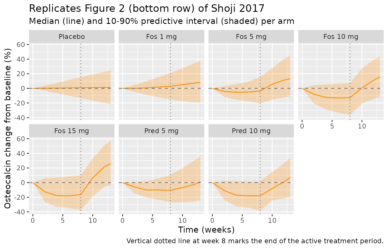
Replicate Table 3: simulated median OC %CFB at week 8
published_table3 <- tibble::tribble(
  ~arm,         ~published_median_pct,
  "Placebo",                       1.8,
  "Fos 1 mg",                      0.1,
  "Fos 5 mg",                     -6.7,
  "Fos 10 mg",                   -12.6,
  "Fos 15 mg",                   -16.8,
  "Pred 5 mg",                    -9.7,
  "Pred 10 mg",                  -16.9
)

simulated_table3 <- sim |>
  group_by(id, arm) |>
  summarise(
    oc_baseline = first(OC[time == 0]),
    oc_week8    = first(OC[time == 8]),
    cfb_pct     = 100 * (oc_week8 - oc_baseline) / oc_baseline,
    .groups = "drop"
  ) |>
  group_by(arm) |>
  summarise(simulated_median_pct = median(cfb_pct, na.rm = TRUE),
            .groups = "drop")

comparison <- published_table3 |>
  left_join(simulated_table3, by = "arm") |>
  mutate(arm = factor(arm, levels = arm_order)) |>
  arrange(arm) |>
  mutate(delta = simulated_median_pct - published_median_pct)

comparison |>
  dplyr::rename(
    "Arm"                             = arm,
    "Published median %CFB (Table 3)" = published_median_pct,
    "Simulated median %CFB"           = simulated_median_pct,
    "Difference (pp)"                 = delta
  ) |>
  knitr::kable(digits = 1,
caption = "Osteocalcin percent change from baseline at week 8 -- published vs simulated.")| Arm | Published median %CFB (Table 3) | Simulated median %CFB | Difference (pp) |
|---|---|---|---|
| Placebo | 1.8 | 1.4 | -0.4 |
| Fos 1 mg | 0.1 | 0.0 | -0.1 |
| Fos 5 mg | -6.7 | -7.0 | -0.3 |
| Fos 10 mg | -12.6 | -11.6 | 1.0 |
| Fos 15 mg | -16.8 | -17.6 | -0.8 |
| Pred 5 mg | -9.7 | -8.4 | 1.3 |
| Pred 10 mg | -16.9 | -14.8 | 2.1 |
Typical-value parameter-recovery checks
sim_typ_summary <- sim_typ |>
  filter(time %in% c(0, 8)) |>
  group_by(arm, time) |>
  summarise(OC_typ = first(OC), .groups = "drop") |>
  pivot_wider(names_from = time, values_from = OC_typ, names_prefix = "wk") |>
  mutate(cfb_pct_typ = 100 * (wk8 - wk0) / wk0,
         arm = factor(arm, levels = arm_order)) |>
  arrange(arm)

sim_typ_summary |>
  dplyr::rename(
    "Arm"               = arm,
    "OC wk 0 (typical)" = wk0,
    "OC wk 8 (typical)" = wk8,
    "%CFB typical"      = cfb_pct_typ
  ) |>
  knitr::kable(digits = 2,
caption = "Typical-value (zero-RE) osteocalcin at week 8 per arm.")| Arm | OC wk 0 (typical) | OC wk 8 (typical) | %CFB typical |
|---|---|---|---|
| Placebo | 22.2 | 22.74 | 2.43 |
| Fos 1 mg | 22.2 | 22.20 | -0.01 |
| Fos 5 mg | 22.2 | 20.44 | -7.93 |
| Fos 10 mg | 22.2 | 18.87 | -15.01 |
| Fos 15 mg | 22.2 | 17.72 | -20.16 |
| Pred 5 mg | 22.2 | 19.71 | -11.20 |
| Pred 10 mg | 22.2 | 17.77 | -19.95 |
Expected typical responses:
- Placebo: OC = BL + SLP * 8 = 22.2 + 0.0675 * 8 = 22.74 ng/mL.
- Fosdagrocorat 10 mg q.d.: ~ -13% CFB at week 8 (paper Discussion / Table 3).
Assumptions and deviations
-
Observation variable naming. The single-output
observation is named
OC(the paper’s name) rather than the canonicalCc. Same accepted deviation as the P1NP sister model and the wider codebase pattern for paper-named biomarker outputs. -
Drug arm switching via reparameterization. Same
convention as the P1NP sister model (base = fosdagrocorat;
dlkel_predanddledk50_predlog-ratio offsets recover the published prednisone values whenDRUG_PRED = 1). For OC the typical-value KDE is fixed to the P1NP estimates – bothlkelanddlkel_predare wrapped infixed(). -
Imax fixed to 1 for both drugs. The OC fit set
Imax = 1for both fosdagrocorat and prednisone because the unconstrained estimate was close to 1 (paper Discussion). The inhibition term1 - imax * ir^c / (edk50^c + ir^c)therefore approaches 0 (full inhibition) at very high IR; the typical OC %CFB at week 8 for the 15 mg fosdagrocorat arm (-16.8% published; ~ -17% simulated) reflects this nearly-complete inhibition combined with the slow OC turnover (Kd = 0.939 /week, longer half-life than the 8-week treatment window). -
Independent (non-block) IIV. Shoji 2017 used
independent IIVs on KDE, EDK50, BL for the OC fit (paper Methods: “To
reduce estimation instability, individual random effect parameters for
KDE, EDK50, and BL were assumed to be independent.”). The model encodes
this with three diagonal
etal*declarations (no block). The IIV CV%s for KDE in OC (123%) are larger than for KDE in P1NP (95%) because the OC fit fits g_KDE to OC residuals alone; this is the paper’s published value and is preserved here. - Taper-period dosing approximation. Same approximation as the P1NP vignette (zero-order rates of 3.5 and 2.33 doses/week of the reduced dose for weeks 8-10 and 10-12).