Levamlodipine (Li 2025)
Source:vignettes/articles/Li_2025_levamlodipine.Rmd
Li_2025_levamlodipine.RmdModel and source
- Citation: Li G, Guan Y, Yang Y, Xiang Q, Chen S, Shao J, Chen Y, Yu X. Model-Informed Precision Dosing of Levamlodipine Besylate in Smoking Patients. Drug Des Devel Ther. 2025;19:3193-3207. doi:10.2147/DDDT.S501762
- Description: One-compartment population PK model with first-order absorption (ka fixed) and a direct-effect inhibitory Imax PD model with baseline for systolic blood pressure after oral levamlodipine besylate once daily in 43 Chinese adults with hypertension (9 smokers, 34 non-smokers) sampled at steady-state trough (Li 2025). Apparent clearance scales as a power of serum uric acid (exponent -0.69, reference 311.0 umol/L) and of MDRD eGFR (exponent 0.95, reference 90.5 mL/min/1.73 m^2); smoking, plasma nicotine and the CYP1A1, CYP1A2, CYP2A6, CYP3A4 and CYP3A5 polymorphisms were screened and not retained. SBP = E0 - Imax * Cc / (IC50 + Cc). The paper reports exponential inter-individual variability on V, CL, E0, Imax and IC50 but none of the variances, so all five etas are fixed to zero.
- Article: https://doi.org/10.2147/DDDT.S501762 (open access, PMC12036611)
Li 2025 fitted a population PK/PD model to steady-state trough levamlodipine concentrations and systolic blood pressure (SBP) in hypertensive patients on levamlodipine besylate monotherapy, with the aim of testing whether smoking (plasma nicotine, and polymorphisms of the enzymes that metabolise cigarette polycyclic aromatic hydrocarbons) changes levamlodipine PK or PD. It did not; the retained covariates are serum uric acid and MDRD eGFR, both on apparent clearance. The model was fitted in Phoenix NLME 8.3 with FOCE-ELS.
Population
43 Chinese adults with essential hypertension (Chongqing, NCT05126381) on a fixed long-term levamlodipine besylate monotherapy regimen: 34 non-smokers (7 male, 27 female) and 9 smokers (all male). Mean age 62.3 (non-smokers) and 64 (smokers) years; mean weight 61.1 and 66.1 kg; mean serum uric acid 311.0 and 357.8 umol/L; mean MDRD eGFR 90.5 and 106.5 mL/min/1.73 m^2 (Li 2025 Table 1). Each patient contributed three steady-state trough concentrations (days 1-3, 0-30 min before the daily dose; 125 analysed after excluding two below the limit of quantification) and three SBP readings plus a baseline SBP (129 SBP values; Table 2).
The same information is available programmatically via
readModelDb("Li_2025_levamlodipine")()$population.
Source trace
Every ini() value carries an in-file comment in
inst/modeldb/specificDrugs/Li_2025_levamlodipine.R; the
table collects them.
| Equation / parameter | Value | Source location |
|---|---|---|
| One-compartment, first-order absorption | n/a | Results ‘Base Model’ |
lka (fixed) |
log(0.79) 1/h | Table 5 ‘tvKa’; Methods: fixed to the literature value |
lvc |
log(3383) L | Table 5 ‘tvV’; final-model V equation |
lcl |
log(58.76) L/h | Table 5 ‘tvCl’; final-model CL equation |
e_uric_acid_cl |
-0.69 | Table 5 ‘dCLdUA’; CL equation (UA / 311.0)^-0.69
|
e_crcl_cl |
0.95 | Table 5 ‘dCLdeGFR’; CL equation (eGFR / 90.5)^0.95
|
le0 |
log(168) mmHg | Table 5 ‘tvE0’; E0 equation |
limax |
log(31.1) mmHg | Table 5 ‘tvImax’; Imax equation; unit from Results ‘Base Model’ |
lic50 |
log(1.71) ng/mL | Table 5 ‘tvIC50’; IC50 equation |
SBP = E0 - Imax * C / (IC50 + C) |
n/a | Results ‘Base Model’ (‘direct effect model with baseline values and suppression effects’) |
etalvc, etalcl, etale0,
etalimax, etalic50
|
fixed(0) | Methods equations 1-5 (exponential IIV); variances not reported |
propSd, propSd_sbp
|
0.06 | Table 5 ‘stdev0’ (one proportional residual for the model) |
Virtual cohort
Individual data are not public. The cohort below draws uric acid and eGFR from the Table 1 means and SDs, separately for the non-smoker and smoker strata. Smoking itself is not a model covariate; the strata are kept only because the paper reports its observations by stratum. The per-patient levamlodipine dose is not reported, so every subject receives 2.5 mg once daily, the lower of the two doses the paper’s Discussion simulates (see Assumptions and deviations).
set.seed(20250425)
n_per_group <- 150

make_cohort <- function(n, group, ua_mean, ua_sd, egfr_mean, egfr_sd, id_offset) {
  # Log-normal uric acid with the Table 1 mean and SD; eGFR normal, truncated to
  # the 30-150 mL/min/1.73 m^2 range a monotherapy outpatient cohort plausibly spans.
  ua_sdlog <- sqrt(log(1 + (ua_sd / ua_mean)^2))
  ua_meanlog <- log(ua_mean) - ua_sdlog^2 / 2
  tibble(
    id = id_offset + seq_len(n),
    group = group,
    URIC_ACID = rlnorm(n, ua_meanlog, ua_sdlog),
    CRCL = pmin(pmax(rnorm(n, egfr_mean, egfr_sd), 30), 150)
  )
}

cohort <- bind_rows(
  make_cohort(n_per_group, "Non-smoker", 311.0, 101.20, 90.46, 17.60, 0L),
  make_cohort(n_per_group, "Smoker", 357.8, 116.70, 106.45, 20.15, n_per_group)
)

dose_mg <- 2.5
tau <- 24
n_doses <- 9 # doses at 0-192 h; troughs at 168, 192 and 216 h as in Figures 8-9
dose_times <- seq(0, by = tau, length.out = n_doses)
obs_times <- sort(unique(c(seq(0, 216, by = 1), seq(192, 216, by = 0.25))))

build_events <- function(cohort, dose_mg) {
  doses <- tidyr::crossing(cohort, time = dose_times) |>
    mutate(evid = 1L, amt = dose_mg, cmt = "depot", dvid = NA_integer_)
  # Two declared endpoints (Cc, sbp): observation rows sit on the central
  # state with dvid = 1, and every row returns both Cc and sbp.
  obs <- tidyr::crossing(cohort, time = obs_times) |>
    mutate(evid = 0L, amt = 0, cmt = "central", dvid = 1L)
  bind_rows(doses, obs) |>
    arrange(id, time, desc(evid))
}

events <- build_events(cohort, dose_mg)
stopifnot(!anyDuplicated(unique(events[events$evid == 1, c("id", "time")])))
Simulation
All five IIV variances are fixed to zero (none is reported), so the
spread below comes only from the uric-acid and eGFR covariates. Model
predictions (Cc, sbp) are used throughout; the
6% proportional residual is not added.
mod <- readModelDb("Li_2025_levamlodipine")
sim <- rxode2::rxSolve(
  mod,
  events = events,
  keep = c("group", "URIC_ACID", "CRCL")
) |>
  as.data.frame()
#> ℹ omega/sigma items treated as zero: 'etalvc', 'etalcl', 'etale0', 'etalimax', 'etalic50'
#> Warning: multi-subject simulation without without 'omega'

troughs <- sim |>
  filter(time %in% c(168, 192, 216)) |>
  mutate(day = factor(time, c(168, 192, 216), c("D1", "D2", "D3")))
Typical-value check
At the reference covariates (uric acid 311.0 umol/L, eGFR 90.5) the model’s day-9 trough after 2.5 mg once daily is compared against the closed-form one-compartment oral solution summed over the nine doses. The two sides use the same parameters, so the check is purely numerical and a tight bound is right.
ka <- 0.79
vc <- 3383
cl <- 58.76
kel <- cl / vc

typ_events <- tibble(id = 1L, URIC_ACID = 311.0, CRCL = 90.5) |>
  build_events(dose_mg = dose_mg)
typ <- rxode2::rxSolve(rxode2::zeroRe(mod), events = typ_events) |>
  as.data.frame()
#> ℹ omega/sigma items treated as zero: 'etalvc', 'etalcl', 'etale0', 'etalimax', 'etalic50'

typ_trough_216 <- typ$Cc[typ$time == 216]
# Superposition of the nine doses: with a 40-h half-life
# (log(2) * 3383 / 58.76 = 39.9 h) nine doses are close to, not at, steady state.
analytic_9 <- sum(
  1000 * dose_mg * ka / (vc * (ka - kel)) *
    (exp(-kel * (216 - dose_times)) - exp(-ka * (216 - dose_times)))
)
stopifnot(abs(typ_trough_216 / analytic_9 - 1) < 1e-4)

typ_sbp_216 <- typ$sbp[typ$time == 216]
stopifnot(abs(typ_sbp_216 - (168 - 31.1 * typ_trough_216 / (1.71 + typ_trough_216))) < 1e-6)
c(trough_ng_mL = typ_trough_216, sbp_mmHg = typ_sbp_216)
#> trough_ng_mL     sbp_mmHg
#>     1.426673   153.854591
The typical trough of about 1.43 ng/mL matches the Table 2 mean day-3 trough of the non-smokers (1.45 ng/mL), supporting the 2.5 mg dose assumption and the PK parameters. The typical SBP of 154 mmHg does not match the paper: see the PD section below.
Replicate published figures
Trough concentrations (Figure 8)
# Replicates Figure 8 of Li 2025: PK VPC of the three steady-state troughs.
# Figure 8 plots concentrations in mg/mL (1E-6 = 1 ng/mL); its predicted median
# lies at about 1.1-1.3 ng/mL and its 90% prediction band spans about
# 0.4-3.9 ng/mL.
troughs |>
  group_by(time) |>
  summarise(
    Q05 = quantile(Cc, 0.05),
    Q50 = median(Cc),
    Q95 = quantile(Cc, 0.95),
    .groups = "drop"
  ) |>
  ggplot(aes(time, Q50)) +
  geom_ribbon(aes(ymin = Q05, ymax = Q95), alpha = 0.25) +
  geom_line() +
  geom_point() +
  coord_cartesian(ylim = c(0, 5)) +
  labs(
    x = "Time after first dose (h)", y = "Levamlodipine trough (ng/mL)",
    title = "Figure 8: steady-state troughs, 2.5 mg once daily",
    caption = "Median and 5th-95th percentiles; covariate-driven spread only (IIV not reported). Replicates Figure 8 of Li 2025."
  )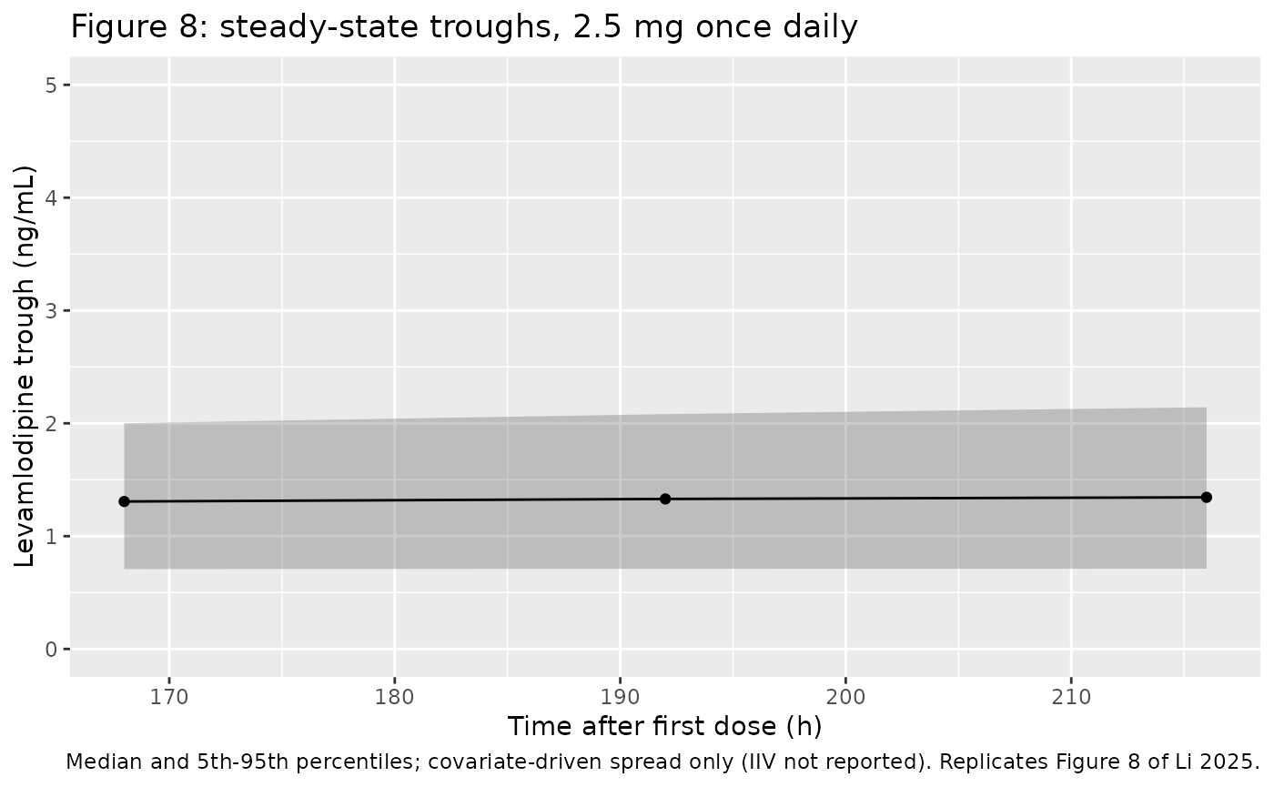
The simulated band is narrower than the published one because the paper’s IIV and the residual error are not in the simulation; the median sits where Figure 8 puts it.
Systolic blood pressure (Figure 9)
# Replicates Figure 9 of Li 2025: PD VPC of SBP at the three troughs. Figure 9's
# predicted median is about 133-135 mmHg.
troughs |>
  group_by(time) |>
  summarise(
    Q05 = quantile(sbp, 0.05),
    Q50 = median(sbp),
    Q95 = quantile(sbp, 0.95),
    .groups = "drop"
  ) |>
  ggplot(aes(time, Q50)) +
  geom_ribbon(aes(ymin = Q05, ymax = Q95), alpha = 0.25) +
  geom_line() +
  geom_point() +
  geom_hline(yintercept = 135, linetype = "dashed", colour = "firebrick") +
  coord_cartesian(ylim = c(110, 180)) +
  labs(
    x = "Time after first dose (h)", y = "SBP (mmHg)",
    title = "Figure 9: SBP at steady-state trough, 2.5 mg once daily",
    caption = "Solid: model median and 5th-95th percentiles. Dashed: approximate Figure 9 predicted median. Replicates Figure 9 of Li 2025."
  )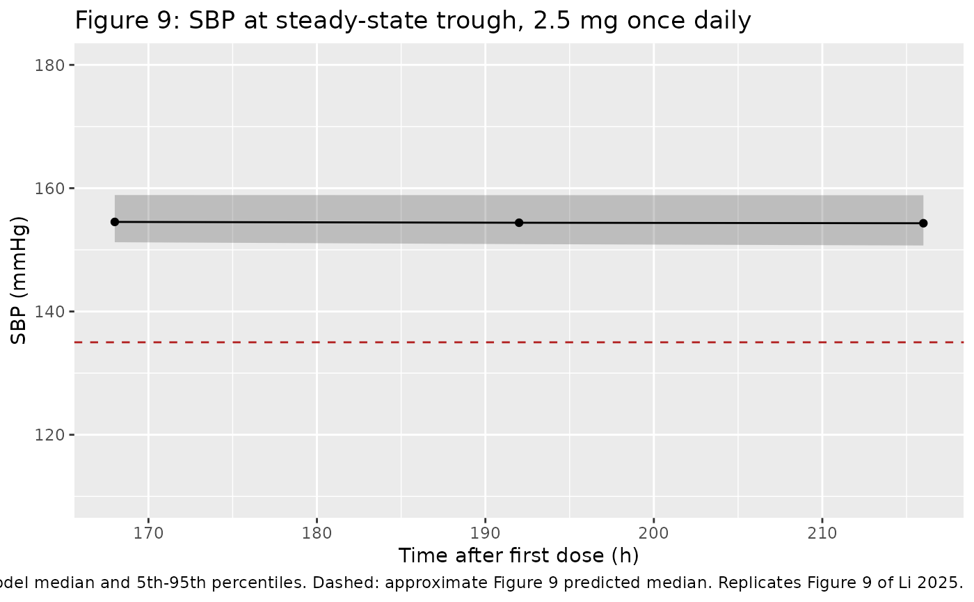
The published PD parameters do not reproduce the published PD fit. With E0 = 168 mmHg, Imax = 31.1 mmHg and IC50 = 1.71 ng/mL, a trough of 1.45 ng/mL gives SBP = 168 - 31.1 x 1.45 / (1.71 + 1.45) = 153.7 mmHg, about 19 mmHg above the Figure 9 predicted median and above every observed mean in Table 2 (128-142 mmHg on treatment). Even the full Imax only lowers SBP to 136.9 mmHg. The model is shipped exactly as printed (Table 5 and the final-model equations); no parameter has been adjusted to close the gap.
sim_sbp_obs <- troughs |>
  group_by(group, day) |>
  summarise(
    `Simulated trough (ng/mL)` = mean(Cc),
    `Simulated SBP (mmHg)` = mean(sbp),
    .groups = "drop"
  )
published_t2 <- tribble(
  ~group, ~day, ~`Observed trough (ng/mL)`, ~`Observed SBP (mmHg)`,
  "Non-smoker", "D1", 1.60, 136,
  "Non-smoker", "D2", 1.49, 131,
  "Non-smoker", "D3", 1.45, 128,
  "Smoker", "D1", 1.71, 142,
  "Smoker", "D2", 1.60, 135,
  "Smoker", "D3", 1.52, 136
)
sim_sbp_obs |>
  mutate(day = as.character(day)) |>
  left_join(published_t2, by = c("group", "day")) |>
  rename("Group" = group, "Day" = day) |>
  knitr::kable(
    digits = 2,
    caption = "Simulated means (2.5 mg once daily) versus the observed means of Li 2025 Table 2."
)| Group | Day | Simulated trough (ng/mL) | Simulated SBP (mmHg) | Observed trough (ng/mL) | Observed SBP (mmHg) |
|---|---|---|---|---|---|
| Non-smoker | D1 | 1.39 | 154.29 | 1.60 | 136 |
| Non-smoker | D2 | 1.43 | 154.14 | 1.49 | 131 |
| Non-smoker | D3 | 1.45 | 154.03 | 1.45 | 128 |
| Smoker | D1 | 1.24 | 155.24 | 1.71 | 142 |
| Smoker | D2 | 1.26 | 155.12 | 1.60 | 135 |
| Smoker | D3 | 1.28 | 155.04 | 1.52 | 136 |
PKNCA validation
The paper reports no NCA. PKNCA is used on the last dosing interval (192-216 h) to summarise steady-state exposure by stratum, and the steady-state minimum is compared with the day-3 observed trough means of Table 2.
sim_nca <- sim |>
  filter(time >= 192, !is.na(Cc)) |>
  select(id, time, Cc, group)

conc_obj <- PKNCA::PKNCAconc(sim_nca, Cc ~ time | group + id)
dose_df <- events |>
  filter(evid == 1) |>
  select(id, time, amt, group)
dose_obj <- PKNCA::PKNCAdose(dose_df, amt ~ time | group + id)
intervals <- data.frame(
  start = 192, end = 216,
  cmax = TRUE, tmax = TRUE, cmin = TRUE, auclast = TRUE, cav = TRUE
)
nca_res <- PKNCA::pk.nca(PKNCA::PKNCAdata(conc_obj, dose_obj, intervals = intervals))

nca_summary <- as.data.frame(nca_res) |>
  filter(PPTESTCD %in% c("cmax", "tmax", "cmin", "auclast", "cav")) |>
  group_by(group, PPTESTCD) |>
  summarise(median = median(PPORRES), .groups = "drop") |>
  tidyr::pivot_wider(names_from = PPTESTCD, values_from = median)
nca_summary |>
  rename(
    "Group" = group, "Cmax (ng/mL)" = cmax, "Tmax (h)" = tmax,
    "Cmin (ng/mL)" = cmin, "AUC0-24 (ng*h/mL)" = auclast, "Cav (ng/mL)" = cav
  ) |>
knitr::kable(digits = 2, caption = "Simulated steady-state NCA (median per stratum), 2.5 mg once daily.")| Group | AUC0-24 (ng*h/mL) | Cav (ng/mL) | Cmax (ng/mL) | Cmin (ng/mL) | Tmax (h) |
|---|---|---|---|---|---|
| Non-smoker | 41.94 | 1.75 | 2.01 | 1.43 | 3.5 |
| Smoker | 36.90 | 1.54 | 1.80 | 1.22 | 3.5 |
published_cmin <- data.frame(group = c("Non-smoker", "Smoker"), cmin = c(1.45, 1.52))
cmp <- nlmixr2lib::ncaComparisonTable(
  simulated = nca_res,
  reference = published_cmin,
  by = "group",
  params = "cmin",
  units = c(cmin = "ng/mL"),
  tolerance_pct = 20
)
cmp |>
  rename("Group" = group) |>
knitr::kable(caption = "Simulated median steady-state Cmin versus the Li 2025 Table 2 day-3 mean trough (observed, unknown per-patient dose).")| NCA parameter | Group | Reference | Simulated | % diff |
|---|---|---|---|---|
| Cmin (ng/mL) | Non-smoker | 1.45 | 1.43 | -1.7% |
| Cmin (ng/mL) | Smoker | 1.52 | 1.22 | -19.6% |
sim_cmin <- as.data.frame(nca_res) |>
  filter(PPTESTCD == "cmin", group == "Non-smoker")
# Centre, not extremes: a mis-transcribed CL, V or covariate reference moves the
# whole distribution by tens of percent.
stopifnot(abs(median(sim_cmin$PPORRES) / 1.45 - 1) < 0.25)
The non-smoker trough is reproduced. The smokers’ simulated trough is about 15-20% lower than the non-smokers’, because their higher mean eGFR (106 vs 90 mL/min/1.73 m^2) raises clearance by more than their higher uric acid lowers it, whereas the observed smoker troughs are slightly higher (Table 2). The gap to the smoker means (about 20%) is well inside the Table 2 SDs (0.76-0.98 ng/mL on means of 1.5-1.7) for nine patients whose individual doses are unknown; smoking itself was tested and not retained in the model.
Dosing scenarios from the Discussion
The Discussion considers 2.5 and 5.0 mg once daily across eGFR 60-120 mL/min/1.73 m^2. The typical-value steady-state troughs and the SBP they imply under the published PD parameters are below.
scen <- tidyr::crossing(
  CRCL = c(60, 90.5, 120),
  dose = c(2.5, 5.0)
) |>
  mutate(id = row_number(), URIC_ACID = 311.0)
scen_events <- bind_rows(lapply(split(scen, scen$id), function(s) {
  build_events(select(s, id, URIC_ACID, CRCL), dose_mg = s$dose)
})) |>
  left_join(select(scen, id, dose), by = "id")
scen_sim <- rxode2::rxSolve(rxode2::zeroRe(mod), events = scen_events, keep = c("dose", "CRCL")) |>
  as.data.frame() |>
  filter(time == 216)
#> ℹ omega/sigma items treated as zero: 'etalvc', 'etalcl', 'etale0', 'etalimax', 'etalic50'
#> Warning: multi-subject simulation without without 'omega'
scen_sim |>
  transmute(
    "eGFR (mL/min/1.73 m^2)" = CRCL, "Dose (mg)" = dose,
    "Trough (ng/mL)" = Cc, "SBP at trough (mmHg)" = sbp
  ) |>
knitr::kable(digits = 2, caption = "Typical-value steady-state trough and SBP (uric acid 311.0 umol/L).")| eGFR (mL/min/1.73 m^2) | Dose (mg) | Trough (ng/mL) | SBP at trough (mmHg) |
|---|---|---|---|
| 60.0 | 2.5 | 2.12 | 150.79 |
| 60.0 | 5.0 | 4.24 | 145.84 |
| 90.5 | 2.5 | 1.43 | 153.85 |
| 90.5 | 5.0 | 2.85 | 148.55 |
| 120.0 | 2.5 | 1.04 | 156.22 |
| 120.0 | 5.0 | 2.08 | 150.92 |
Assumptions and deviations
-
IIV variances not reported. Methods equations 1-5
place exponential IIV on V, CL, E0, Imax and IC50, but no omega is
reported anywhere in the paper. All five etas are
fixed(0); simulations show only covariate-driven spread. -
One residual error for two endpoints. Table 5
reports a single proportional
stdev0= 0.06 for a model with two observed variables (concentration and SBP; Figures 8 and 9). It is applied to both endpoints. - Conflicting typical values. Table 5 and the printed final-model equations give V = 3383 L and CL = 58.76 L/h. Table 6 (‘Final model’ column) gives 3572 L and 59.61 L/h, and the abstract 3521 L and 62.6 L/h (which are the base-model values quoted in the Results text, although Table 4 prints the base model as 3383 / 58.76). The model follows Table 5 and the equations.
- PD parameters do not reproduce the PD fit. See the Figure 9 section: the printed E0 / Imax / IC50 give a typical on-treatment SBP of about 154 mmHg against a published predicted median of about 135 mmHg. Imax is entered in mmHg as the Results text states. The Discussion’s statement that 2.5 mg keeps SBP below 140 mmHg from a baseline of 165 mmHg also cannot be reproduced with these values. The model is shipped as printed.
- eGFR effect in the Discussion. The Discussion states that an eGFR of 60 mL/min/1.73 m^2 gives a CL of about 46.94% of the typical value; the printed power term gives (60 / 90.5)^0.95 = 67.7%. The printed equation is followed.
- Sign of the uric-acid effect. The abstract says patients with lower uric acid had lower CL, which implies a positive exponent; Table 5, Table 6 and the printed equation all give -0.69, which is used.
- Dose. The per-patient dose is not reported. 2.5 mg once daily is used for the cohort; at the reference covariates it reproduces the observed mean day-3 trough of the non-smokers.
-
eGFR column. The paper’s MDRD eGFR (Chinese MDRD
form printed under Table 1, BSA-normalised) is supplied as the canonical
CRCLcolumn. - Covariate distributions. Uric acid is drawn log-normal and eGFR normal (truncated to 30-150) from the Table 1 means and SDs per stratum; the paper gives no ranges.