Repotrectinib exposure-response (Du 2025)
Source:vignettes/articles/Du_2025_repotrectinib_exposure_response.Rmd
Du_2025_repotrectinib_exposure_response.RmdDu S, Hu Z, Shen J, Zhu L, Roy A, Lam J, Lu M, Kondic A, Hamuro L. Exposure-Response Analysis of Repotrectinib to Support the Dose Recommendation for Patients With ROS1-Positive NSCLC or NTRK-Positive Solid Tumors. CPT Pharmacometrics Syst Pharmacol. 2025;14(12):1993-2005. doi:10.1002/psp4.70102
Repotrectinib is a ROS1 / TRK / ALK tyrosine kinase inhibitor dosed
at 160 mg once daily for 14 days and then 160 mg twice daily (“160 mg
QD/BID”). Du 2025 relates exposure from TRIDENT-1 to efficacy and safety
with nine independently fitted regressions. All nine are packaged here,
and each takes its exposure metric as a data column. Those metrics come
from the companion population PK model of the same group (Du 2025, doi:10.1002/psp4.70036),
which the package already carries as Du_2025_repotrectinib.
This vignette uses that model to generate the exposures.
| Model | Endpoint | Form | Exposure driver |
|---|---|---|---|
Du_2025_repotrectinib_orr_ros1 |
Confirmed objective response, ROS1+ NSCLC | logistic | log Cavg56 |
Du_2025_repotrectinib_orr_ntrk |
Confirmed objective response, NTRK+ solid tumors | logistic | log Cavg56 |
Du_2025_repotrectinib_pfs_ros1 |
Progression-free survival, ROS1+ NSCLC | Cox | log Cavgc (time-varying) |
Du_2025_repotrectinib_pfs_ntrk |
Progression-free survival, NTRK+ solid tumors | Cox | log Cavgc (time-varying) |
Du_2025_repotrectinib_dizziness_grade2 |
Grade >= 2 dizziness | Cox | Cavgc (time-varying) |
Du_2025_repotrectinib_anemia_grade2 |
Grade >= 2 anemia | Cox | Cavgc (time-varying) |
Du_2025_repotrectinib_teae_grade3 |
Grade >= 3 treatment-emergent AE | Cox | Cavgc (time-varying) |
Du_2025_repotrectinib_neae_grade2 |
Grade >= 2 neurologic AE | Cox | Cavgc (time-varying) |
Du_2025_repotrectinib_drdi |
Dose reduction or interruption due to an AE | Cox | Cavgc (time-varying) |
Cavg56 is the average concentration over the first 56 days of treatment. Cavgc is the cumulative average concentration from day 1 to the current time, AUC(0, t) / t, updated every half day. Both are in ng/mL.
mods <- c(
  "orr_ros1", "orr_ntrk", "pfs_ros1", "pfs_ntrk", "dizziness_grade2",
  "anemia_grade2", "teae_grade3", "neae_grade2", "drdi"
)
er <- lapply(
  setNames(paste0("Du_2025_repotrectinib_", mods), mods),
  function(nm) rxode2::rxode2(readModelDb(nm))
)
Population
All data come from the single-arm phase 1/2 TRIDENT-1 trial (NCT03093116; data cutoff March 2023). The efficacy models were fitted separately by indication: 127 adults with ROS1-positive NSCLC (124 evaluable for response) and 88 adults with NTRK1-3-fusion-positive solid tumors (83 evaluable for response). The safety models pool 502 adults with ROS1-, NTRK- or ALK-positive tumors (Du 2025 Tables S1 and S2).
| ROS1+ NSCLC | NTRK+ solid tumors | Safety set | |
|---|---|---|---|
| N | 127 | 88 | 502 |
| Age, median (range), years | 57 (28-80) | 60 (20-84) | 56 (18-93) |
| Weight, median (range), kg | 63.5 (39.5-119.3) | 70 (42-116.3) | 69 (39.5-169.4) |
| Female | 63.8% | 53.4% | 56.5% (Figure 5) |
| Asian | 59.1% | 37.5% | 47.0% |
| ECOG PS 1 | 66.9% | 58.0% | 65.3% (Figure 5) |
| TKI-pretreated | 44.1% | 54.5% | 65.7% |
| Baseline tumor size, median, cm | 4.9 | 5.7 | 5.1 |
| On 160 mg QD/BID | 92% | 91% | 84% |
Source trace
Every coefficient is a printed estimate. The ORR models come from
Table S6, the PFS models from Table S10, and the safety models from
Table S14. Each ini() line names its table row. The two
logistic intercepts are the only values not printed by the paper. They
are back-solved below.
| Element | Source |
|---|---|
Logistic structure, logit(p) = gamma0 + gamma X
|
Methods, Equation 1; Table S5 formulas (uncentred
rms::lrm) |
Cox structure, h(t) = h0(t) exp(beta X)
|
Methods, Equation 2; Tables S9 and S13 formulas |
| Exposure functional form (log Cavg56; log Cavgc for PFS; linear Cavgc for safety) | Tables S5, S9 and S13 (lowest-BIC models) |
| ORR coefficients | Table S6 |
| PFS coefficients | Table S10 |
| Safety coefficients | Table S14 |
| Forest-plot reference values used for centring the Cox models | Figures 3 and 5 |
logit_ref (both ORR models) |
Back-solved from Table S1 response counts; see the next section |
| Exposures in this vignette |
Du_2025_repotrectinib (doi:10.1002/psp4.70036) |
Recovering the logistic intercepts
The paper prints the slope of every ORR covariate but not the intercept. For a maximum-likelihood logistic regression with an intercept, the score equation forces the fitted probabilities to sum to the number of observed responders. This holds overall and within every level of a dummy covariate. The intercept is therefore the value that makes the mean fitted probability, over the analysis set’s covariate distribution, equal the observed response rate. Here that distribution is reconstructed from the Table S1 summaries and the Figure 1 exposure percentiles, with covariates drawn independently.
expit <- function(x) 1 / (1 + exp(-x))
solve_g0 <- function(rest, target) {
  uniroot(function(g) mean(expit(g + rest)) - target, c(-30, 30))$root
}
set.seed(1)
n <- 200000
lnorm_mean_cv <- function(n, mean, cv) {
  s <- sqrt(log(1 + cv^2))
  rlnorm(n, log(mean) - s^2 / 2, s)
}

# ROS1+ NSCLC: Table S1 totals; Figure 1A Cavg56 median 273, P5-P95 136-523
lc <- rnorm(n, log(273), (log(523) - log(136)) / (2 * qnorm(0.95)))
rest_ros1 <- 1.551 * lc - 0.0113 * rnorm(n, 55.6, 12.4) -
  0.0118 * lnorm_mean_cv(n, 65.4, 14.1 / 65.4) -
  0.01916 * lnorm_mean_cv(n, 6.1, 4.3 / 6.1) +
  0.1005 * rbinom(n, 1, 80 / 124) - 0.4202 * rbinom(n, 1, 72 / 124) -
  0.138 * rbinom(n, 1, 83 / 124)
tki <- rbinom(n, 1, 55 / 124)
g_ros1 <- c(
  overall = solve_g0(rest_ros1 - 1.92 * tki, 77 / 124),
  naive = solve_g0(rest_ros1, 56 / 69),
  pretreated = solve_g0(rest_ros1 - 1.92, 21 / 55)
)

# NTRK+ solid tumors: Table S1 totals; Figure 1B Cavg56 median 257, P5-P95
# 79-478; NTRK3 prevalence by TKI stratum from the Table S11 column counts.
lc <- rnorm(n, log(257), (log(478) - log(79)) / (2 * qnorm(0.95)))
rest_ntrk <- 0.2871 * lc - 0.03726 * rnorm(n, 55.6, 15.6) +
  0.01421 * lnorm_mean_cv(n, 71.2, 16.3 / 71.2) -
  0.07697 * lnorm_mean_cv(n, 7.2, 5.5 / 7.2) +
  0.3882 * rbinom(n, 1, 46 / 83) + 0.7497 * rbinom(n, 1, 30 / 83) -
  0.1154 * rbinom(n, 1, 47 / 83) - 0.3631 * rbinom(n, 1, 53 / 88)
n3_naive <- rbinom(n, 1, 18 / 40)
n3_pre <- rbinom(n, 1, 33 / 48)
tki <- rbinom(n, 1, 46 / 83)
g_ntrk <- c(
  overall = solve_g0(
    rest_ntrk + 2.259 * ifelse(tki == 1, n3_pre, n3_naive) - 1.054 * tki,
    47 / 83
  ),
  naive = solve_g0(rest_ntrk + 2.259 * n3_naive, 23 / 37),
  pretreated = solve_g0(rest_ntrk + 2.259 * n3_pre - 1.054, 24 / 46)
)
round(rbind(ROS1 = g_ros1, NTRK = g_ntrk), 3)
#>      overall  naive pretreated
#> ROS1  -5.424 -5.303     -5.527
#> NTRK  -0.565 -0.488     -0.622

shipped <- c(
  ROS1 = unname(rxode2::rxode2(er$orr_ros1)$theta["logit_ref"]),
  NTRK = unname(rxode2::rxode2(er$orr_ntrk)$theta["logit_ref"])
)
shipped
#>  ROS1  NTRK
#> -5.42 -0.56
# The packaged values are the overall solutions, rounded to 0.01.
stopifnot(abs(shipped - c(g_ros1[["overall"]], g_ntrk[["overall"]])) < 0.02)
The two within-stratum solutions differ by 0.2 logit (ROS1) and 0.1 logit (NTRK). That spread is the cost of drawing covariates that were correlated in the trial as if they were independent. The packaged intercept is the overall solution.
Forest-plot reproduction
The odds and hazard ratios in Figures 1, 3 and 5 at the covariate P5 and P95 values follow directly from the coefficients and the printed reference values. This check is deterministic. The packaged model is evaluated at the reference patient and at the shifted patient, and the ratio of the outputs is compared with the printed value.
# One observation row per scenario; the static models have no time axis, so
# time is only an index.
er_eval <- function(model, output, covs) {
  ev <- data.frame(id = 1L, time = seq_len(nrow(covs)), amt = 0, evid = 0L)
  ev <- cbind(ev, covs)
  s <- as.data.frame(rxode2::rxSolve(model, events = ev, returnType = "data.frame"))
  stopifnot(nrow(s) == nrow(covs))
  s[[output]]
}
odds <- function(p) p / (1 - p)
ref_ros1 <- data.frame(
  CAV = 273, AGE = 57, WT = 64, TUMSZ = 49, SEXF = 0, RACE_ASIAN = 0,
  ECOG_GE1 = 0, PRIOR_TKI = 0
)
ref_ntrk <- data.frame(
  CAV = 257, AGE = 60, WT = 70, TUMSZ = 57, SEXF = 0, RACE_ASIAN = 0,
  ECOG_GE1 = 0, PRIOR_TKI = 0, TUM_NTRK3_MUT = 0, TUMTP_OTHER = 0
)
ref_safety <- data.frame(
  CAV = 300, AGE = 56, WT = 69, SEXF = 1, RACE_ASIAN = 0, RACE_OTHER = 0,
  ECOG_GE1 = 1, PRIOR_TKI = 1, TUM_NTRK_MUT = 0, TUM_ALK_MUT = 0,
  TUMTP_OTHER = 0
)
shift <- function(ref, ...) {
  x <- ref
  v <- list(...)
  x[names(v)] <- v
  x
}
ratio <- function(model, ref, kind, ...) {
  new <- shift(ref, ...)
  if (kind == "OR") {
    p <- er_eval(model, "prob_orr", rbind(ref, new))
    odds(p[2]) / odds(p[1])
  } else {
    h <- er_eval(model, "hr", rbind(ref, new))
    h[2] / h[1]
  }
}

forest <- bind_rows(
  tibble(
    figure = "1A ORR ROS1",
    row = c("TKI pretreated:naive", "Cavg56 P05 136", "Cavg56 P95 523",
            "Age P05 35", "Weight P95 89", "Tumor size P05 1.44"),
    printed = c(0.147, 0.338, 2.74, 1.28, 0.745, 1.07),
    model = c(
      ratio(er$orr_ros1, ref_ros1, "OR", PRIOR_TKI = 1),
      ratio(er$orr_ros1, ref_ros1, "OR", CAV = 136),
      ratio(er$orr_ros1, ref_ros1, "OR", CAV = 523),
      ratio(er$orr_ros1, ref_ros1, "OR", AGE = 35),
      ratio(er$orr_ros1, ref_ros1, "OR", WT = 89),
      ratio(er$orr_ros1, ref_ros1, "OR", TUMSZ = 14.4)
    )
  ),
  tibble(
    figure = "1B ORR NTRK",
    row = c("NTRK3:NTRK1-2", "Others:NSCLC", "Cavg56 P05 79",
            "Cavg56 P95 478", "Age P05 27", "Tumor size P95 17"),
    printed = c(9.57, 0.696, 0.713, 1.19, 3.42, 0.419),
    model = c(
      ratio(er$orr_ntrk, ref_ntrk, "OR", TUM_NTRK3_MUT = 1),
      ratio(er$orr_ntrk, ref_ntrk, "OR", TUMTP_OTHER = 1),
      ratio(er$orr_ntrk, ref_ntrk, "OR", CAV = 79),
      ratio(er$orr_ntrk, ref_ntrk, "OR", CAV = 478),
      ratio(er$orr_ntrk, ref_ntrk, "OR", AGE = 27),
      ratio(er$orr_ntrk, ref_ntrk, "OR", TUMSZ = 170)
    )
  ),
  tibble(
    figure = "3A PFS ROS1",
    row = c("TKI pretreated:naive", "Sex female:male", "Tumor size P95 14.7",
            "Weight P05 45.1", "Age P95 75"),
    printed = c(4.48, 0.463, 2.3, 1.4, 1.07),
    model = c(
      ratio(er$pfs_ros1, ref_ros1, "HR", PRIOR_TKI = 1),
      ratio(er$pfs_ros1, ref_ros1, "HR", SEXF = 1),
      ratio(er$pfs_ros1, ref_ros1, "HR", TUMSZ = 147),
      ratio(er$pfs_ros1, ref_ros1, "HR", WT = 45.1),
      ratio(er$pfs_ros1, ref_ros1, "HR", AGE = 75)
    )
  ),
  tibble(
    figure = "3B PFS NTRK",
    row = c("NTRK3:NTRK1-2", "TKI pretreated:naive", "Tumor size P95 17",
            "Age P05 27", "Weight P95 96.1"),
    printed = c(0.311, 3.43, 1.87, 0.591, 0.953),
    model = c(
      ratio(er$pfs_ntrk, ref_ntrk, "HR", TUM_NTRK3_MUT = 1),
      ratio(er$pfs_ntrk, ref_ntrk, "HR", PRIOR_TKI = 1),
      ratio(er$pfs_ntrk, ref_ntrk, "HR", TUMSZ = 170),
      ratio(er$pfs_ntrk, ref_ntrk, "HR", AGE = 27),
      ratio(er$pfs_ntrk, ref_ntrk, "HR", WT = 96.1)
    )
  ),
  tibble(
    figure = "5A Gr2+ dizziness",
    row = c("Age P05 32", "Age P95 75", "Weight P95 105",
            "TKI naive:pretreated", "PS fully active:restricted"),
    printed = c(0.301, 2.59, 0.896, 1.24, 0.652),
    model = c(
      ratio(er$dizziness_grade2, ref_safety, "HR", AGE = 32),
      ratio(er$dizziness_grade2, ref_safety, "HR", AGE = 75),
      ratio(er$dizziness_grade2, ref_safety, "HR", WT = 105),
      ratio(er$dizziness_grade2, ref_safety, "HR", PRIOR_TKI = 0),
      ratio(er$dizziness_grade2, ref_safety, "HR", ECOG_GE1 = 0)
    )
  ),
  tibble(
    figure = "5B DRDI",
    row = c("Age P95 75", "Weight P05 47.8", "Weight P95 105",
            "NTRK:ROS1", "Race others:White"),
    printed = c(1.64, 0.729, 1.71, 1.63, 1.52),
    model = c(
      ratio(er$drdi, ref_safety, "HR", AGE = 75),
      ratio(er$drdi, ref_safety, "HR", WT = 47.8),
      ratio(er$drdi, ref_safety, "HR", WT = 105),
      ratio(er$drdi, ref_safety, "HR", TUM_NTRK_MUT = 1),
      ratio(er$drdi, ref_safety, "HR", RACE_OTHER = 1)
    )
  )
) |>
  mutate(pct_diff = 100 * (model / printed - 1))

forest |>
  mutate(model = signif(model, 3), pct_diff = round(pct_diff, 2)) |>
  rename(
    "Figure" = figure, "Ratio" = row, "Printed" = printed,
    "Packaged model" = model, "Difference (%)" = pct_diff
  ) |>
knitr::kable()| Figure | Ratio | Printed | Packaged model | Difference (%) |
|---|---|---|---|---|
| 1A ORR ROS1 | TKI pretreated:naive | 0.147 | 0.147 | -0.27 |
| 1A ORR ROS1 | Cavg56 P05 136 | 0.338 | 0.339 | 0.40 |
| 1A ORR ROS1 | Cavg56 P95 523 | 2.740 | 2.740 | 0.04 |
| 1A ORR ROS1 | Age P05 35 | 1.280 | 1.280 | 0.17 |
| 1A ORR ROS1 | Weight P95 89 | 0.745 | 0.745 | -0.06 |
| 1A ORR ROS1 | Tumor size P05 1.44 | 1.070 | 1.070 | -0.14 |
| 1B ORR NTRK | NTRK3:NTRK1-2 | 9.570 | 9.570 | 0.04 |
| 1B ORR NTRK | Others:NSCLC | 0.696 | 0.696 | -0.07 |
| 1B ORR NTRK | Cavg56 P05 79 | 0.713 | 0.713 | -0.04 |
| 1B ORR NTRK | Cavg56 P95 478 | 1.190 | 1.200 | 0.42 |
| 1B ORR NTRK | Age P05 27 | 3.420 | 3.420 | -0.01 |
| 1B ORR NTRK | Tumor size P95 17 | 0.419 | 0.419 | 0.01 |
| 3A PFS ROS1 | TKI pretreated:naive | 4.480 | 4.480 | -0.06 |
| 3A PFS ROS1 | Sex female:male | 0.463 | 0.463 | -0.08 |
| 3A PFS ROS1 | Tumor size P95 14.7 | 2.300 | 2.300 | -0.01 |
| 3A PFS ROS1 | Weight P05 45.1 | 1.400 | 1.400 | -0.16 |
| 3A PFS ROS1 | Age P95 75 | 1.070 | 1.070 | 0.40 |
| 3B PFS NTRK | NTRK3:NTRK1-2 | 0.311 | 0.311 | 0.10 |
| 3B PFS NTRK | TKI pretreated:naive | 3.430 | 3.430 | -0.06 |
| 3B PFS NTRK | Tumor size P95 17 | 1.870 | 1.870 | -0.08 |
| 3B PFS NTRK | Age P05 27 | 0.591 | 0.591 | 0.06 |
| 3B PFS NTRK | Weight P95 96.1 | 0.953 | 0.953 | 0.02 |
| 5A Gr2+ dizziness | Age P05 32 | 0.301 | 0.301 | -0.03 |
| 5A Gr2+ dizziness | Age P95 75 | 2.590 | 2.590 | -0.09 |
| 5A Gr2+ dizziness | Weight P95 105 | 0.896 | 0.896 | 0.00 |
| 5A Gr2+ dizziness | TKI naive:pretreated | 1.240 | 1.240 | -0.15 |
| 5A Gr2+ dizziness | PS fully active:restricted | 0.652 | 0.652 | 0.05 |
| 5B DRDI | Age P95 75 | 1.640 | 1.640 | 0.06 |
| 5B DRDI | Weight P05 47.8 | 0.729 | 0.729 | -0.02 |
| 5B DRDI | Weight P95 105 | 1.710 | 1.710 | 0.06 |
| 5B DRDI | NTRK:ROS1 | 1.630 | 1.630 | 0.13 |
| 5B DRDI | Race others:White | 1.520 | 1.520 | 0.27 |
# Deterministic: only the paper's three-significant-figure rounding separates
# the two columns.
stopifnot(all(abs(forest$pct_diff) < 1.5))
The text gives three further dose-independent safety contrasts. For grade >= 2 anemia, the hazard ratio at 47.6 versus 69 kg is 1.74. For grade >= 2 neurologic AEs, the hazard ratios are 1.41 at 75 versus 56 years and 1.84 at 105 versus 69 kg.
txt <- tibble(
  contrast = c("Anemia, weight 47.6 vs 69 kg", "NEAE, age 75 vs 56",
               "NEAE, weight 105 vs 69 kg", "TEAE grade 3, male vs female"),
  printed = c(1.74, 1.41, 1.84, 1.34),
  model = c(
    ratio(er$anemia_grade2, ref_safety, "HR", WT = 47.6),
    ratio(er$neae_grade2, ref_safety, "HR", AGE = 75),
    ratio(er$neae_grade2, ref_safety, "HR", WT = 105),
    ratio(er$teae_grade3, ref_safety, "HR", SEXF = 0)
  )
)
knitr::kable(txt, digits = 3)| contrast | printed | model |
|---|---|---|
| Anemia, weight 47.6 vs 69 kg | 1.74 | 1.736 |
| NEAE, age 75 vs 56 | 1.41 | 1.406 |
| NEAE, weight 105 vs 69 kg | 1.84 | 1.838 |
| TEAE grade 3, male vs female | 1.34 | 1.340 |
Exposure simulation
Table S7 (ORR) and Table S11 (PFS) report predictions for six regimens: 40, 80, 120 and 200 mg QD/BID, 160 mg QD and 160 mg QD/BID, all with unknown prandial state. To reproduce them, exposures are simulated from the companion popPK model with its between-subject variability. Two virtual adult cohorts of 150 patients each are drawn from the Table S1 covariate summaries, one per indication. A cumulative-AUC state is piped into the PK model, so Cavg56 and Cavgc(t) are both read off as AUC(0, t) / t. Within a cohort, every regimen reuses the same subjects and the same random-number seed, so the regimens differ only by dose.
# The companion model selects its clearance eta by cohort (healthy volunteer
# or patient), which rxode2 reports as "non-mu referenced" whenever the model
# is parsed; that parameterisation is deliberate, so only that message is
# muffled.
muffle_mu_ref <- function(w) {
  if (grepl("non-mu referenced", conditionMessage(w))) {
    invokeRestart("muffleWarning")
  }
}
pk <- withCallingHandlers(
  rxode2::rxode2(readModelDb("Du_2025_repotrectinib")),
  warning = muffle_mu_ref
)
# append = Cc places the accumulator after the line that computes Cc.
pk_auc <- withCallingHandlers(
  rxode2::model(pk, d/dt(auc) <- Cc, append = Cc),
  warning = muffle_mu_ref
)
n_sub <- 150
rtrunc <- function(n, mean, sd, lo, hi) {
  x <- rnorm(n, mean, sd)
  pmin(pmax(x, lo), hi)
}
make_cohort <- function(seed, age, wt, ts, female, asian, ps1) {
  set.seed(seed)
  s_wt <- sqrt(log(1 + (wt[2] / wt[1])^2))
  s_ts <- sqrt(log(1 + (ts[2] / ts[1])^2))
  tibble(
    id = seq_len(n_sub),
    AGE = rtrunc(n_sub, age[1], age[2], age[3], age[4]),
    WT = pmin(pmax(rlnorm(n_sub, log(wt[1]) - s_wt^2 / 2, s_wt), wt[3]), wt[4]),
    TUMSZ = 10 * rlnorm(n_sub, log(ts[1]) - s_ts^2 / 2, s_ts),
    SEXF = rbinom(n_sub, 1, female),
    RACE_ASIAN = rbinom(n_sub, 1, asian),
    ECOG_GE1 = rbinom(n_sub, 1, ps1)
  )
}
# Table S1 totals: mean, SD, min, max (age); mean, SD, min, max (weight);
# mean, SD (tumor size, cm).
cohort_ros1 <- make_cohort(
  101, c(55.6, 12.4, 28, 80), c(65.4, 14.1, 39.5, 119.3), c(6.1, 4.3),
  80 / 124, 72 / 124, 83 / 124
)
cohort_ntrk <- make_cohort(
  202, c(55.6, 15.6, 20, 84), c(71.2, 16.3, 42, 116.3), c(7.2, 5.5),
  46 / 83, 30 / 83, 47 / 83
) |>
  mutate(TUMTP_OTHER = rbinom(n_sub, 1, 53 / 88))
regimens <- tribble(
  ~regimen, ~dose, ~bid,
  "40 mg QD/BID", 40, TRUE,
  "80 mg QD/BID", 80, TRUE,
  "120 mg QD/BID", 120, TRUE,
  "160 mg QD", 160, FALSE,
  "160 mg QD/BID", 160, TRUE,
  "200 mg QD/BID", 200, TRUE
)
obs_days <- c(56, 91, 182, 365)

sim_exposure <- function(cohort, dose, bid) {
  t_end <- 24 * max(obs_days)
  ev <- if (bid) {
    rxode2::et(amt = dose, ii = 24, until = 24 * 13, cmt = "depot") |>
      rxode2::et(amt = dose, time = 24 * 14, ii = 12, until = t_end - 1,
                 cmt = "depot")
  } else {
    rxode2::et(amt = dose, ii = 24, until = t_end - 1, cmt = "depot")
  }
  ev <- rxode2::et(ev, c(0, 24 * obs_days), cmt = "central") |>
    rxode2::et(id = cohort$id)
  d <- as.data.frame(ev) |>
    left_join(select(cohort, id, WT), by = "id") |>
    mutate(AGE = 50, DIS_HEALTHY = 0, FED = 0, FED_MISSING = 1,
           FASTED_STRICT = 0)
  rxode2::rxSetSeed(2025)
  s <- rxode2::rxSolve(pk_auc, d, returnType = "data.frame",
                       atol = 1e-8, rtol = 1e-6, maxsteps = 1e6)
  # Drop the day-0 row, where AUC / t is undefined; this is not a PKNCA input.
  s <- s[s$time > 0, ]
  transmute(s, id, day = time / 24, cav = auc / time)
}

expo <- bind_rows(lapply(c("ros1", "ntrk"), function(ind) {
  cohort <- if (ind == "ros1") cohort_ros1 else cohort_ntrk
  bind_rows(lapply(seq_len(nrow(regimens)), function(i) {
    sim_exposure(cohort, regimens$dose[i], regimens$bid[i]) |>
      mutate(indication = ind, regimen = regimens$regimen[i])
  }))
})) |>
  mutate(regimen = factor(regimen, levels = regimens$regimen))

stopifnot(!anyNA(expo$cav))

expo |>
  filter(day %in% c(56, 365)) |>
  group_by(indication, regimen, day) |>
  summarise(median = median(cav), .groups = "drop") |>
  pivot_wider(names_from = c(indication, day), values_from = median) |>
  rename(
    "Regimen" = regimen,
    "ROS1 Cavg56" = ros1_56, "ROS1 Cavgc day 365" = ros1_365,
    "NTRK Cavg56" = ntrk_56, "NTRK Cavgc day 365" = ntrk_365
  ) |>
knitr::kable(digits = 0, caption = "Median simulated exposure (ng/mL).")| Regimen | NTRK Cavg56 | NTRK Cavgc day 365 | ROS1 Cavg56 | ROS1 Cavgc day 365 |
|---|---|---|---|---|
| 40 mg QD/BID | 117 | 123 | 114 | 121 |
| 80 mg QD/BID | 200 | 206 | 195 | 204 |
| 120 mg QD/BID | 273 | 279 | 267 | 276 |
| 160 mg QD | 251 | 239 | 241 | 231 |
| 160 mg QD/BID | 340 | 346 | 336 | 343 |
| 200 mg QD/BID | 404 | 409 | 401 | 407 |
At 160 mg QD/BID the simulated median Cavg56 sits above the Figure 1 analysis set medians (273 and 257 ng/mL). That is the expected direction: the analysis set includes the dose interruptions and reductions recorded in the trial, and the nominal-regimen simulation has none.
PKNCA check of the exposure metric
Cavg56 here comes from an integrated AUC state. As an independent check, PKNCA computes AUC(0-56 days) with its default linear-up/log-down trapezoidal rule on an hourly profile for a subset of the ROS1 cohort at 160 mg QD/BID. The PKNCA formula groups by regimen.
n_nca <- 20
ev <- rxode2::et(amt = 160, ii = 24, until = 24 * 13, cmt = "depot") |>
  rxode2::et(amt = 160, time = 24 * 14, ii = 12, until = 24 * 56 - 1,
             cmt = "depot") |>
  rxode2::et(seq(0, 24 * 56, by = 1), cmt = "central") |>
  rxode2::et(id = seq_len(n_nca))
d <- as.data.frame(ev) |>
  left_join(select(cohort_ros1, id, WT), by = "id") |>
  mutate(AGE = 50, DIS_HEALTHY = 0, FED = 0, FED_MISSING = 1,
         FASTED_STRICT = 0)
rxode2::rxSetSeed(2025)
s_nca <- rxode2::rxSolve(pk_auc, d, returnType = "data.frame",
                         atol = 1e-8, rtol = 1e-6, maxsteps = 1e6) |>
  mutate(treatment = "160 mg QD/BID")

conc <- s_nca |>
  filter(!is.na(Cc)) |>
  select(id, time, Cc, treatment)
dose_df <- d |>
  filter(evid == 1) |>
  mutate(treatment = "160 mg QD/BID") |>
  select(id, time, amt, treatment)
o_conc <- PKNCAconc(conc, Cc ~ time | treatment + id)
o_dose <- PKNCAdose(dose_df, amt ~ time | treatment + id)
o_data <- PKNCAdata(
  o_conc, o_dose,
  intervals = data.frame(start = 0, end = 24 * 56, auclast = TRUE)
)
nca <- as.data.frame(pk.nca(o_data))

cmp <- nca |>
  filter(PPTESTCD == "auclast") |>
  transmute(id, cavg_pknca = PPORRES / (24 * 56)) |>
  left_join(
    s_nca |> filter(time == 24 * 56) |> transmute(id, cavg_ode = auc / time),
    by = "id"
  ) |>
  mutate(pct_diff = 100 * (cavg_pknca / cavg_ode - 1))
summary(cmp$pct_diff)
#>    Min. 1st Qu.  Median    Mean 3rd Qu.    Max.
#> 0.05536 0.41710 0.59010 0.62449 0.90712 1.29091
# Same drawn parameters on both sides, so the difference is pure quadrature
# error: an hourly grid clips the narrow absorption peaks of the fast
# absorbers, and the trapezoid overstates AUC by up to about 1.3%.
stopifnot(
  abs(median(cmp$pct_diff)) < 1,
  all(abs(cmp$pct_diff) < 2.5)
)
Objective response: Table S7
Every virtual patient is evaluated twice, as TKI-naive and as TKI-pretreated. NTRK patients are also evaluated as NTRK1-2 and as NTRK3. The resulting medians are compared with the medians the paper predicts in Table S7. Because the logit is monotone, the median predicted probability equals the probability at the median linear predictor. The two medians are therefore directly comparable on the logit scale.
orr_pred <- function(indication, model, extra) {
  cohort <- if (indication == "ros1") cohort_ros1 else cohort_ntrk
  base <- expo |>
    filter(indication == !!indication, day == 56) |>
    left_join(cohort, by = "id")
  bind_rows(lapply(seq_len(nrow(extra)), function(j) {
    x <- base
    for (nm in names(extra)) x[[nm]] <- extra[[nm]][j]
    covs <- as.data.frame(select(x, -id, -day, -indication, -regimen))
    names(covs)[names(covs) == "cav"] <- "CAV"
    mutate(x, prob = er_eval(model, "prob_orr", covs))
  }))
}
orr_ros1 <- orr_pred("ros1", er$orr_ros1, tibble(PRIOR_TKI = c(0, 1))) |>
  mutate(group = ifelse(PRIOR_TKI == 1, "ROS1 TKI-pretreated", "ROS1 TKI-naive"))
orr_ntrk <- orr_pred(
  "ntrk", er$orr_ntrk,
  expand_grid(PRIOR_TKI = c(0, 1), TUM_NTRK3_MUT = c(0, 1))
) |>
  mutate(group = paste0(
    "NTRK", ifelse(TUM_NTRK3_MUT == 1, "3", "1-2"), " ",
    ifelse(PRIOR_TKI == 1, "TKI-pretreated", "TKI-naive")
  ))

# Table S7 medians. The NTRK values are listed in the column order of
# Table S11 (naive NTRK1-2, naive NTRK3, pretreated NTRK1-2, pretreated
# NTRK3); see the Errata for why Table S7's own NTRK headers are not used.
s7 <- tribble(
  ~regimen, ~`ROS1 TKI-naive`, ~`ROS1 TKI-pretreated`, ~`NTRK1-2 TKI-naive`,
  ~`NTRK3 TKI-naive`, ~`NTRK1-2 TKI-pretreated`, ~`NTRK3 TKI-pretreated`,
  "40 mg QD/BID", 0.524, 0.146, 0.327, 0.836, 0.185, 0.636,
  "80 mg QD/BID", 0.713, 0.278, 0.361, 0.855, 0.209, 0.670,
  "120 mg QD/BID", 0.801, 0.383, 0.382, 0.866, 0.223, 0.689,
  "160 mg QD", 0.761, 0.331, 0.372, 0.861, 0.216, 0.679,
  "160 mg QD/BID", 0.850, 0.466, 0.397, 0.873, 0.235, 0.702,
  "200 mg QD/BID", 0.882, 0.533, 0.409, 0.879, 0.244, 0.713
) |>
  pivot_longer(-regimen, names_to = "group", values_to = "published")

orr_cmp <- bind_rows(orr_ros1, orr_ntrk) |>
  group_by(regimen, group) |>
  summarise(simulated = median(prob), .groups = "drop") |>
  mutate(regimen = as.character(regimen)) |>
  inner_join(s7, by = c("regimen", "group")) |>
  mutate(
    logit_diff = qlogis(simulated) - qlogis(published),
    indication = ifelse(grepl("^ROS1", group), "ROS1", "NTRK")
  )
stopifnot(nrow(orr_cmp) == 36)

orr_cmp |>
  mutate(across(c(simulated, published), \(x) round(x, 3)),
         logit_diff = round(logit_diff, 2)) |>
  arrange(group, factor(regimen, levels = regimens$regimen)) |>
  select(group, regimen, published, simulated, logit_diff) |>
  rename(
    "Subgroup" = group, "Regimen" = regimen,
    "Table S7 median Pr(OR)" = published, "Simulated median Pr(OR)" = simulated,
    "Logit difference" = logit_diff
  ) |>
knitr::kable()| Subgroup | Regimen | Table S7 median Pr(OR) | Simulated median Pr(OR) | Logit difference |
|---|---|---|---|---|
| NTRK1-2 TKI-naive | 40 mg QD/BID | 0.327 | 0.331 | 0.02 |
| NTRK1-2 TKI-naive | 80 mg QD/BID | 0.361 | 0.366 | 0.02 |
| NTRK1-2 TKI-naive | 120 mg QD/BID | 0.382 | 0.387 | 0.02 |
| NTRK1-2 TKI-naive | 160 mg QD | 0.372 | 0.382 | 0.04 |
| NTRK1-2 TKI-naive | 160 mg QD/BID | 0.397 | 0.402 | 0.02 |
| NTRK1-2 TKI-naive | 200 mg QD/BID | 0.409 | 0.414 | 0.02 |
| NTRK1-2 TKI-pretreated | 40 mg QD/BID | 0.185 | 0.147 | -0.27 |
| NTRK1-2 TKI-pretreated | 80 mg QD/BID | 0.209 | 0.168 | -0.27 |
| NTRK1-2 TKI-pretreated | 120 mg QD/BID | 0.223 | 0.181 | -0.26 |
| NTRK1-2 TKI-pretreated | 160 mg QD | 0.216 | 0.177 | -0.25 |
| NTRK1-2 TKI-pretreated | 160 mg QD/BID | 0.235 | 0.190 | -0.27 |
| NTRK1-2 TKI-pretreated | 200 mg QD/BID | 0.244 | 0.198 | -0.27 |
| NTRK3 TKI-naive | 40 mg QD/BID | 0.836 | 0.826 | -0.07 |
| NTRK3 TKI-naive | 80 mg QD/BID | 0.855 | 0.847 | -0.06 |
| NTRK3 TKI-naive | 120 mg QD/BID | 0.866 | 0.858 | -0.07 |
| NTRK3 TKI-naive | 160 mg QD | 0.861 | 0.856 | -0.05 |
| NTRK3 TKI-naive | 160 mg QD/BID | 0.873 | 0.866 | -0.07 |
| NTRK3 TKI-naive | 200 mg QD/BID | 0.879 | 0.871 | -0.07 |
| NTRK3 TKI-pretreated | 40 mg QD/BID | 0.636 | 0.623 | -0.06 |
| NTRK3 TKI-pretreated | 80 mg QD/BID | 0.670 | 0.659 | -0.05 |
| NTRK3 TKI-pretreated | 120 mg QD/BID | 0.689 | 0.678 | -0.05 |
| NTRK3 TKI-pretreated | 160 mg QD | 0.679 | 0.674 | -0.02 |
| NTRK3 TKI-pretreated | 160 mg QD/BID | 0.702 | 0.692 | -0.05 |
| NTRK3 TKI-pretreated | 200 mg QD/BID | 0.713 | 0.702 | -0.05 |
| ROS1 TKI-naive | 40 mg QD/BID | 0.524 | 0.518 | -0.03 |
| ROS1 TKI-naive | 80 mg QD/BID | 0.713 | 0.716 | 0.01 |
| ROS1 TKI-naive | 120 mg QD/BID | 0.801 | 0.804 | 0.02 |
| ROS1 TKI-naive | 160 mg QD | 0.761 | 0.783 | 0.13 |
| ROS1 TKI-naive | 160 mg QD/BID | 0.850 | 0.852 | 0.02 |
| ROS1 TKI-naive | 200 mg QD/BID | 0.882 | 0.883 | 0.01 |
| ROS1 TKI-pretreated | 40 mg QD/BID | 0.146 | 0.136 | -0.08 |
| ROS1 TKI-pretreated | 80 mg QD/BID | 0.278 | 0.269 | -0.04 |
| ROS1 TKI-pretreated | 120 mg QD/BID | 0.383 | 0.376 | -0.03 |
| ROS1 TKI-pretreated | 160 mg QD | 0.331 | 0.346 | 0.07 |
| ROS1 TKI-pretreated | 160 mg QD/BID | 0.466 | 0.459 | -0.03 |
| ROS1 TKI-pretreated | 200 mg QD/BID | 0.533 | 0.525 | -0.03 |
ggplot(orr_cmp, aes(regimen, simulated, colour = group, group = group)) +
  geom_line() +
  geom_point() +
  geom_point(aes(y = published), shape = 4, size = 3) +
  facet_wrap(~indication) +
  labs(x = NULL, y = "Median predicted Pr(OR)", colour = NULL) +
  theme_bw() +
  theme(axis.text.x = element_text(angle = 30, hjust = 1),
        legend.position = "bottom")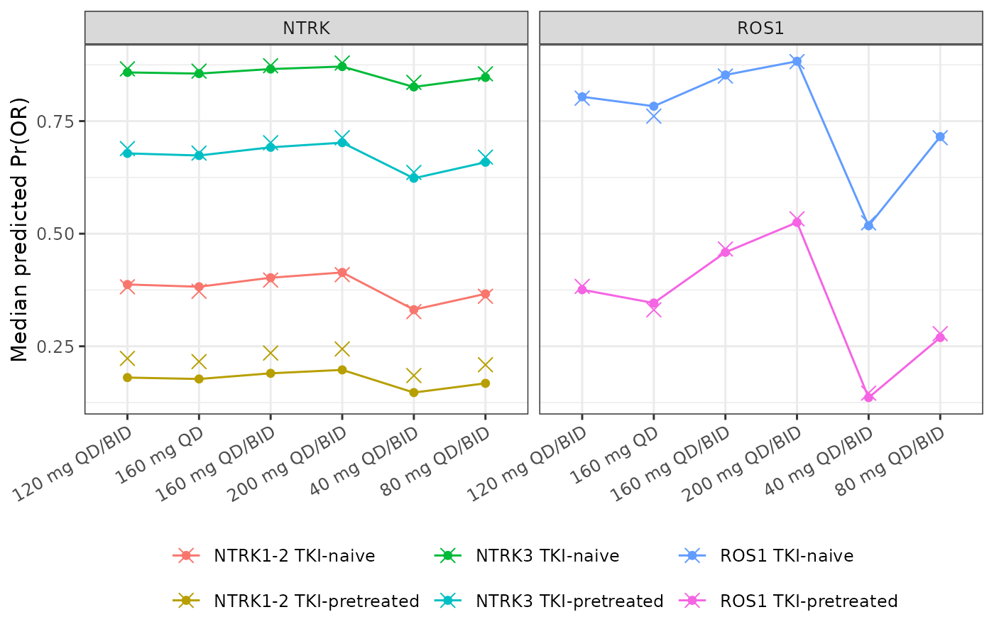
Replicates Figure 2A of Du 2025: median predicted probability of objective response by regimen (points: simulated; crosses: Table S7).
orr_cmp |>
  group_by(indication) |>
  summarise(
    median_logit_diff = median(logit_diff),
    max_abs_logit_diff = max(abs(logit_diff))
  )
#> # A tibble: 2 × 3
#>   indication median_logit_diff max_abs_logit_diff
#>   <chr>                  <dbl>              <dbl>
#> 1 NTRK                -0.0541               0.274
#> 2 ROS1                -0.00848              0.126
ros1 <- filter(orr_cmp, indication == "ROS1")
ntrk <- filter(orr_cmp, indication == "NTRK")
naive_at <- function(r) {
  qlogis(ros1$simulated[ros1$group == "ROS1 TKI-naive" & ros1$regimen == r])
}
span_sim <- naive_at("200 mg QD/BID") - naive_at("40 mg QD/BID")
span_pub <- qlogis(0.882) - qlogis(0.524)
c(simulated = span_sim, published = span_pub)
#> simulated published
#>  1.949956  1.915434
stopifnot(
  # ROS1: the back-solved intercept and the simulated exposures together
  # reproduce the paper's own predictions at the centre.
  abs(median(ros1$logit_diff)) < 0.2,
  quantile(abs(ros1$logit_diff), 0.9) < 0.4,
  # NTRK: centre as tight as ROS1; the tail is wider because the NTRK1-2
  # pretreated column of Table S7 averages over its own 15 patients (see the
  # PFS section and Errata).
  abs(median(ntrk$logit_diff)) < 0.2,
  quantile(abs(ntrk$logit_diff), 0.9) < 0.4,
  # The exposure slope: the 40 mg to 200 mg span of the ROS1 TKI-naive curve.
  abs(span_sim - span_pub) < 0.4
)
Both indications match Table S7 at the centre: the median logit difference is about 0.01 (ROS1) and 0.05 (NTRK). The predictions are driven by the companion popPK model, and the ROS1 exposure slope is the printed 1.551. Matching the absolute level checks the back-solved intercepts against a source they were not derived from: Table S7 holds the authors’ own model predictions, and the intercepts came from the observed response counts in Table S1. One subgroup, NTRK1-2 TKI-pretreated, sits about 0.27 logit (4 percentage points) below Table S7 at every regimen. Each Table S7 column was simulated over that column’s own patients (the 15 NTRK1-2 pretreated patients), while this vignette uses one shared virtual cohort for all four NTRK columns. The PFS section below finds the same column-specific shift in Table S11.
Progression-free survival: Table S11
A Cox model carries no baseline hazard, so the absolute PFS
probabilities in Table S11 cannot be regenerated. What Table S11 does
pin are the hazard contrasts. Within a column, the median
survival at time t is S = exp(-H0(t) * exp(lhr)) evaluated
at the median linear predictor. The log-cumulative-hazard difference
log(-log S_a) - log(-log S_b) between two columns or two
regimens is therefore the difference of their linear predictors.
s11 <- tribble(
  ~month, ~regimen, ~ros1_naive, ~ros1_pre, ~n12_naive, ~n3_naive, ~n12_pre, ~n3_pre,
  3, "40 mg QD/BID", 0.921, 0.696, 0.735, 0.915, 0.400, 0.732,
  3, "80 mg QD/BID", 0.952, 0.805, 0.791, 0.934, 0.497, 0.788,
  3, "120 mg QD/BID", 0.964, 0.852, 0.818, 0.943, 0.552, 0.816,
  3, "160 mg QD", 0.963, 0.847, 0.818, 0.942, 0.545, 0.812,
  3, "160 mg QD/BID", 0.971, 0.878, 0.836, 0.949, 0.589, 0.834,
  3, "200 mg QD/BID", 0.975, 0.896, 0.848, 0.953, 0.617, 0.847,
  6, "40 mg QD/BID", 0.835, 0.448, 0.487, 0.812, 0.117, 0.483,
  6, "80 mg QD/BID", 0.897, 0.618, 0.576, 0.852, 0.194, 0.572,
  6, "120 mg QD/BID", 0.922, 0.699, 0.624, 0.872, 0.247, 0.620,
  6, "160 mg QD", 0.916, 0.681, 0.617, 0.866, 0.233, 0.607,
  6, "160 mg QD/BID", 0.936, 0.748, 0.655, 0.884, 0.288, 0.652,
  6, "200 mg QD/BID", 0.945, 0.781, 0.678, 0.894, 0.321, 0.676,
  12, "40 mg QD/BID", 0.668, 0.165, 0.250, 0.669, 0.0158, 0.246,
  12, "80 mg QD/BID", 0.783, 0.339, 0.344, 0.734, 0.0419, 0.340,
  12, "120 mg QD/BID", 0.833, 0.446, 0.401, 0.767, 0.0667, 0.397,
  12, "160 mg QD", 0.817, 0.411, 0.389, 0.754, 0.0574, 0.376,
  12, "160 mg QD/BID", 0.861, 0.519, 0.440, 0.788, 0.0894, 0.437,
  12, "200 mg QD/BID", 0.881, 0.573, 0.471, 0.804, 0.110, 0.468
)
cloglog <- function(s) log(-log(s))
theta <- function(m, p) unname(rxode2::rxode2(m)$theta[p])
cov_contrast <- s11 |>
  transmute(
    month, regimen,
    `ROS1 TKI pretreated vs naive` = cloglog(ros1_pre) - cloglog(ros1_naive),
    `NTRK1-2 TKI pretreated vs naive` = cloglog(n12_pre) - cloglog(n12_naive),
    `NTRK3 TKI pretreated vs naive` = cloglog(n3_pre) - cloglog(n3_naive),
    `TKI-naive NTRK3 vs NTRK1-2` = cloglog(n3_naive) - cloglog(n12_naive),
    `TKI-pretreated NTRK3 vs NTRK1-2` = cloglog(n3_pre) - cloglog(n12_pre)
  ) |>
  pivot_longer(-c(month, regimen), names_to = "contrast", values_to = "table_s11") |>
  mutate(coefficient = case_when(
    grepl("^ROS1", contrast) ~ theta(er$pfs_ros1, "e_prior_tki_haz"),
    grepl("TKI pretreated vs naive", contrast) ~ theta(er$pfs_ntrk, "e_prior_tki_haz"),
    TRUE ~ theta(er$pfs_ntrk, "e_tum_ntrk3_mut_haz")
  ))
cov_contrast |>
  group_by(contrast) |>
  summarise(
    coefficient = first(coefficient),
    `Table S11 median` = median(table_s11),
    `Table S11 range` = paste(round(range(table_s11), 2), collapse = " to ")
  ) |>
  rename("Contrast (log cumulative hazard)" = contrast, "Packaged coefficient" = coefficient) |>
knitr::kable(digits = 3)| Contrast (log cumulative hazard) | Packaged coefficient | Table S11 median | Table S11 range |
|---|---|---|---|
| NTRK1-2 TKI pretreated vs naive | 1.232 | 1.088 | 1.07 to 1.11 |
| NTRK3 TKI pretreated vs naive | 1.232 | 1.248 | 1.24 to 1.26 |
| ROS1 TKI pretreated vs naive | 1.499 | 1.483 | 1.47 to 1.5 |
| TKI-naive NTRK3 vs NTRK1-2 | -1.167 | -1.237 | -1.24 to -1.21 |
| TKI-pretreated NTRK3 vs NTRK1-2 | -1.167 | -1.072 | -1.08 to -1.07 |
stopifnot(
  abs(median(cov_contrast$table_s11 - cov_contrast$coefficient)) < 0.1,
  all(abs(cov_contrast$table_s11 - cov_contrast$coefficient) < 0.25)
)
The ROS1 TKI contrast reproduces the printed coefficient 1.499 to within 0.03 in every cell. The NTRK contrasts scatter by up to 0.17 around their coefficients. Table S11’s column counts (22, 18, 15 and 33 patients) show that each NTRK column was simulated over its own subjects, so their other covariates differ.
# Exposure contrast against 160 mg QD/BID: Table S11 versus the packaged
# coefficient times the simulated difference in median log Cavgc.
month_day <- c(`3` = 91, `6` = 182, `12` = 365)
sim_lcav <- expo |>
  filter(day %in% month_day) |>
  mutate(month = as.numeric(names(month_day)[match(day, month_day)])) |>
  group_by(indication, regimen, month) |>
  summarise(med_lcav = median(log(cav)), .groups = "drop")
ref_lcav <- sim_lcav |>
  filter(regimen == "160 mg QD/BID") |>
  select(indication, month, ref = med_lcav)
pred <- sim_lcav |>
  left_join(ref_lcav, by = c("indication", "month")) |>
  mutate(
    beta = ifelse(indication == "ros1", theta(er$pfs_ros1, "e_cav_haz"),
                  theta(er$pfs_ntrk, "e_cav_haz")),
    predicted = beta * (med_lcav - ref),
    regimen = as.character(regimen)
  )
s11_ref <- s11 |> filter(regimen == "160 mg QD/BID")
obs <- s11 |>
  left_join(s11_ref, by = "month", suffix = c("", "_ref")) |>
  transmute(
    month, regimen,
    ros1 = cloglog(ros1_naive) - cloglog(ros1_naive_ref),
    ntrk = cloglog(n12_naive) - cloglog(n12_naive_ref)
  ) |>
  pivot_longer(c(ros1, ntrk), names_to = "indication", values_to = "table_s11")
expo_contrast <- inner_join(obs, pred, by = c("indication", "month", "regimen")) |>
  filter(regimen != "160 mg QD/BID")
expo_contrast |>
  filter(month == 12) |>
  select(indication, regimen, table_s11, predicted) |>
  rename(
    "Indication" = indication, "Regimen" = regimen,
    "Table S11 (12 months)" = table_s11, "Packaged model" = predicted
  ) |>
  knitr::kable(digits = 3,
caption = "Log cumulative hazard of progression relative to 160 mg QD/BID (TKI-naive; NTRK1-2 column for NTRK).")| Indication | Regimen | Table S11 (12 months) | Packaged model |
|---|---|---|---|
| ros1 | 40 mg QD/BID | 0.992 | 0.983 |
| ntrk | 40 mg QD/BID | 0.524 | 0.516 |
| ros1 | 80 mg QD/BID | 0.491 | 0.492 |
| ntrk | 80 mg QD/BID | 0.262 | 0.258 |
| ros1 | 120 mg QD/BID | 0.200 | 0.204 |
| ntrk | 120 mg QD/BID | 0.107 | 0.107 |
| ros1 | 160 mg QD | 0.300 | 0.373 |
| ntrk | 160 mg QD | 0.140 | 0.184 |
| ros1 | 200 mg QD/BID | -0.167 | -0.161 |
| ntrk | 200 mg QD/BID | -0.087 | -0.084 |
stopifnot(
  abs(median(expo_contrast$table_s11 - expo_contrast$predicted)) < 0.1,
  quantile(abs(expo_contrast$table_s11 - expo_contrast$predicted), 0.9) < 0.25
)
The dose gradient in Table S11 is reproduced by the packaged exposure coefficients applied to the popPK-simulated Cavgc. Lowering the dose from 160 mg QD/BID to 40 mg QD/BID raises the ROS1 log cumulative hazard by about 1. The fourfold dose cut lowers Cavgc only about threefold: the trough-driven autoinduction of clearance is weaker at lower exposure, so exposure falls less than in proportion to dose.
Safety: relative hazard by regimen
The safety models are linear in Cavgc. Figure 6 of the paper shows predicted cumulative event probabilities, which need the unreported baseline hazards. What carries over without them is the relative hazard between regimens for an otherwise identical patient, shown here at day 365 using the ROS1 cohort’s exposures.
safety <- c("dizziness_grade2", "anemia_grade2", "teae_grade3",
            "neae_grade2", "drdi")
med_cav <- expo |>
  filter(indication == "ros1", day == 365) |>
  group_by(regimen) |>
  summarise(cav = median(cav), .groups = "drop")
saf <- bind_rows(lapply(safety, function(m) {
  covs <- ref_safety[rep(1, nrow(med_cav)), ]
  covs$CAV <- med_cav$cav
  h <- er_eval(er[[m]], "hr", covs)
  tibble(endpoint = m, regimen = med_cav$regimen, cav = med_cav$cav,
         rel_hr = h / h[med_cav$regimen == "160 mg QD/BID"])
}))
ggplot(saf, aes(regimen, rel_hr, colour = endpoint, group = endpoint)) +
  geom_hline(yintercept = 1, linetype = 2) +
  geom_line() +
  geom_point() +
  labs(x = NULL, y = "Hazard ratio vs 160 mg QD/BID", colour = NULL) +
  theme_bw() +
  theme(axis.text.x = element_text(angle = 30, hjust = 1),
        legend.position = "bottom")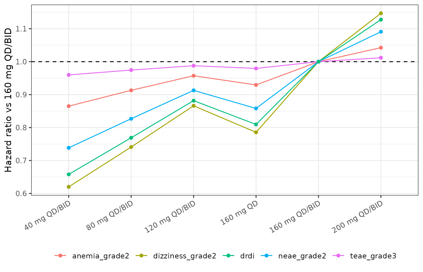
Relative hazard of each safety endpoint against 160 mg QD/BID, at the median simulated Cavgc on day 365 (ROS1 cohort).
saf |>
  filter(regimen %in% c("160 mg QD", "200 mg QD/BID")) |>
  select(endpoint, regimen, rel_hr) |>
  pivot_wider(names_from = regimen, values_from = rel_hr) |>
  rename("Endpoint" = endpoint) |>
knitr::kable(digits = 3)| Endpoint | 160 mg QD | 200 mg QD/BID |
|---|---|---|
| dizziness_grade2 | 0.786 | 1.147 |
| anemia_grade2 | 0.929 | 1.042 |
| teae_grade3 | 0.979 | 1.012 |
| neae_grade2 | 0.858 | 1.091 |
| drdi | 0.809 | 1.128 |
The ordering matches the paper’s account of Figure 6. Dizziness,
neurologic AEs and dose modification rise with dose. Anemia and grade
>= 3 TEAEs are nearly flat. The hazard difference between 160 mg QD
and 160 mg QD/BID is modest. The Discussion quotes cumulative grade
>= 2 dizziness of 15% versus 13% for the two regimens. That pair
corresponds to a hazard ratio of log(0.85) / log(0.87) =
1.17, against 1.27 from the packaged model at the simulated exposures.
The reported percentages are not tied to a stated time point, so this
comparison is illustrative only.
Assumptions and deviations
-
No PK layer in the exposure-response models. Each
model takes its exposure as the
CAVcovariate column: Cavg56 for ORR, and the time-varying Cavgc for PFS and safety. The paper derived both from the empirical Bayes estimates of the companion popPK model and the actual dosing records. This vignette instead simulates nominal regimens fromDu_2025_repotrectinibwith between-subject variability and unknown prandial state, matching the scenario Table S7 and Table S11 describe. - Natural logarithm. The log-exposure terms use the natural log. Figure 1 pins this: the P5 and P95 odds ratios reproduce only with the natural log.
-
Tumor size units. The paper reports baseline tumor
size in cm. The register’s
TUMSZis in mm, so the models divide by 10 and the printed per-cm coefficients are unchanged. - Logistic intercepts. Back-solved as shown above. They are maintainer derivations, not printed values. The two within-stratum solutions differ by 0.1-0.2 logit, which bounds the error from treating the trial covariates as independent. Against Table S7, the centre agrees to within 0.05 logit.
-
Cox models return relative hazards only. The
semiparametric fits never estimate a baseline hazard, and none is
invented here. The ROS1 and NTRK PFS models centre the continuous
covariates on the Figure 3 reference values. The safety models centre
them on the Figure 5 values (56 years, 69 kg). The exposure term is left
uncentred, so
hris relative to a reference patient at Cavgc = 1 ng/mL (PFS) or 0 ng/mL (safety). Centring changes only the baseline hazard, never a hazard ratio. -
Source orientation of categorical safety effects.
Table S14 codes sex as male:female, performance status as 0:1 and prior
TKI as naive:pretreated. The printed coefficients are kept verbatim and
multiply
1 - SEXF,1 - ECOG_GE1and1 - PRIOR_TKI. -
Placeholder residual on the ORR probability. The
source likelihood is Bernoulli. The fixed
addSd_prob_orr = 0.001exists only so rxode2 accepts the observation declaration. - Virtual cohorts. Covariates are drawn independently from the Table S1 marginal summaries (150 per indication). Their joint structure in the trial is not reported.
Errata
- Table S1, responder columns transposed. For both indications, the ORR “Responders” and “Non-responders” headers are swapped. As printed, ROS1 TKI-naive patients would have an ORR of 13/69 (19%) and pretreated patients 34/55 (62%). That contradicts the fitted odds ratio for pretreatment (0.147) and the paper’s own Table S7 predictions. With the headers swapped, the rates are 56/69 (81%) and 21/55 (38%). The NTRK cohort likewise has 47 responders and 36 non-responders, not the reverse. The Results sentence “36 responders and 47 non-responders” repeats the transposition. The intercept back-solve uses the corrected counts.
- Table S7, NTRK column headers. The NTRK columns are printed under NTRK1-2 (naive, pretreated) and NTRK3 (naive, pretreated) spans. Read that way, pretreated patients would respond far better than naive patients, and NTRK1-2 better than NTRK3, which contradicts both odds ratios (0.349 and 9.57). The values instead follow the column order of Table S11: naive NTRK1-2, naive NTRK3, pretreated NTRK1-2, pretreated NTRK3. Read in that order, the logit contrasts reproduce both coefficients.
- Table S2, sex and performance-status rows. Table S2 gives 287 male / 215 female and 326 PS 0 / 176 PS 1. Figure 5 gives 213:277 and 170:320, matching the female and PS 1 majorities of both efficacy subsets. The Figure 5 counts are used in the safety models’ population metadata.
- Footnotes on the exposure scale. Table S3 footnote c reads “for every 100 ng/mL increase in log-form of exposure measure”. Table S6 and Figure 1 show the odds ratio is per unit of natural-log exposure. Table S10 footnote c mentions “Log(Cavg56)” although the PFS models use Cavgc. Both are copy errors with no effect on the estimates.
- Sex orientation in Table S9. The Table S9 abbreviation list codes sex as “Male:Female”, but the Table S10 estimates are labelled “Female: Male”. The Results confirm the Table S10 orientation: female sex lowers the risk of progression in ROS1-positive NSCLC.
- Neurologic AE exposure effect. The paper treats exposure as non-significant for grade >= 2 neurologic AEs (printed hazard-ratio CI 1.000-1.002). The printed estimate and standard error (0.001365, 0.0005416) give z = 2.5, so the rounding of the CI hides a nominally significant effect. The coefficient is packaged as printed.
- Column-specific covariates in Tables S7 and S11. The column counts (71 and 56 ROS1; 22, 18, 15 and 33 NTRK) show that each prediction column was simulated over that column’s own patients. The between-column contrasts therefore mix the coefficient with differences in the other covariates. This shows most in the NTRK1-2 TKI-pretreated column (15 patients), where Table S7 implies a TKI log-odds contrast of -0.76 against the printed -1.054. Table S11 implies a TKI log-hazard contrast of 1.09 against the printed 1.232. The packaged coefficients are the printed ones; neither intercept was tuned to these tables.