Acetaminophen and ibuprofen formulation and food effects (Morse 2022)
Source:vignettes/articles/Morse_2022_acetaminophen_ibuprofen.Rmd
Morse_2022_acetaminophen_ibuprofen.RmdModel and source
Morse 2022 fitted two independent population PK models to the same pooled healthy-volunteer data set, one for acetaminophen and one for ibuprofen. Both are packaged here and share this article.
- Citation: Morse JD, Stanescu I, Atkinson HC, Anderson BJ. Population Pharmacokinetic Modelling of Acetaminophen and Ibuprofen: the Influence of Body Composition, Formulation and Feeding in Healthy Adult Volunteers. Eur J Drug Metab Pharmacokinet. 2022;47(4):497-507. doi:10.1007/s13318-022-00766-9
- Acetaminophen model: Two-compartment population PK model for acetaminophen (paracetamol) in healthy adult volunteers given intravenous, tablet, oral-suspension and sachet formulations of an acetaminophen + ibuprofen combination under fasted and fed conditions (Morse 2022). First-order absorption with a lag time from a depot; absorption half-life and lag time carry formulation-specific factors when fasted and formulation-specific factors when fed, all relative to the fasted tablet. Clearances scale allometrically (exponent 3/4) with normal fat mass (Ffat = 0.816) and volumes linearly with total body weight (Ffat fixed to 1), standardised to a 70 kg, 1.76 m male; fat-free mass is predicted from weight, height and sex (Janmahasatian). Combined additive + proportional residual error with between-subject variability on the residual magnitude.
- Ibuprofen model: Two-compartment population PK model for ibuprofen in healthy adult volunteers given intravenous, tablet, oral-suspension and sachet formulations of an acetaminophen + ibuprofen combination (and intravenous ibuprofen alone) under fasted and fed conditions (Morse 2022). First-order absorption with a lag time from a depot; absorption half-life and lag time carry formulation-specific factors when fasted and formulation-specific factors when fed, all relative to the fasted tablet. Clearances scale allometrically (exponent 3/4) with normal fat mass (Ffat = 0.863) and volumes linearly with normal fat mass (Ffat = 0.718), standardised to a 70 kg, 1.76 m male; fat-free mass is predicted from weight, height and sex (Janmahasatian). Combined additive + proportional residual error with between-subject variability on the residual magnitude.
- Article (open access): https://doi.org/10.1007/s13318-022-00766-9
- Electronic supplementary material (correlation matrices, Table S2; the pharmacodynamic parameters used for the pain-score simulations, Table S3): https://static-content.springer.com/esm/art%3A10.1007%2Fs13318-022-00766-9/MediaObjects/13318_2022_766_MOESM1_ESM.pdf
Population
Data were pooled from four single-centre, single-dose, randomised crossover studies in 116 healthy adults (Morse 2022 Section 2.1): MXIV-01 (n = 30) and MXIV-06 (n = 30) compared intravenous acetaminophen and ibuprofen (alone or combined, 15 min infusions; 30 min for the 400 mg ibuprofen product) with combination tablets, fasted; MX-14a (n = 28) and MX-14b (n = 28) compared the combination as film-coated tablets, ready-to-use oral suspension and a sachet (powder dissolved in 200 mL water), fasted in MX-14a and fed in MX-14b. The pooled participants (Table 1) were 18-49 years old (median 24), weighed 49-116 kg (median 70.8), were 156-199 cm tall (median 173) and 93 were male and 23 female. The analysis used 6095 acetaminophen and 6046 ibuprofen concentrations.
The same information is available programmatically through each
model’s population metadata, e.g.
readModelDb("Morse_2022_ibuprofen")()$population.
Model structure
Both drugs use a two-compartment disposition model with first-order
elimination. Oral doses enter a depot with bioavailability
F, a lag time TLAG and a first-order
absorption rate ka = ln(2) / T1/2ABS; intravenous doses are
infusions into the central compartment.
Size and body composition. Fat-free mass is predicted from
weight, height and sex (Janmahasatian; Eq. 2). Normal fat mass is
NFM = FFM + Ffat * (WT - FFM) (Eqs. 3-4), and each
parameter is scaled by (NFM / NFM_STD)^EXP with
EXP fixed at 3/4 for clearances and 1 for volumes (Eqs. 1
and 5). The standard individual is a 70 kg, 1.76 m male whose FFM is
56.1 kg, so NFM_STD = 56.1 + Ffat * (70 - 56.1).
Acetaminophen uses Ffat = 0.816 for clearances and
Ffat = 1 (total body weight) for volumes; ibuprofen uses
0.863 and 0.718.
Formulation and food. The fasted tablet is the reference for
T1/2ABS and TLAG. In the fasted state the
suspension and the sachet each carry their own factor; in the fed state
each of the three oral formulations carries its own factor, again
relative to the fasted tablet (the fed factor replaces, rather than
multiplies, the fasted formulation factor). The section “Which reference
do the fed factors use?” below shows why.
Residual error is combined additive and proportional with a
between-subject random effect on its magnitude (Eq. 8):
SD = sqrt((Cc * propSd)^2 + addSd^2) * exp(etaRUV).
Source trace
Every ini() value carries an in-file source comment in
inst/modeldb/specificDrugs/Morse_2022_acetaminophen.R and
inst/modeldb/specificDrugs/Morse_2022_ibuprofen.R. They are
collected here.
| Parameter | Acetaminophen | Ibuprofen | Source |
|---|---|---|---|
lcl (CL, L/h/70 kg) |
24.0 | 3.79 | Tables 2 / 3 |
lvc (V1, L/70 kg) |
43.7 | 6.05 | Tables 2 / 3 |
lq (Q2, L/h/70 kg) |
43.5 | 10.5 | Tables 2 / 3 |
lvp (V2, L/70 kg) |
29.7 | 4.37 | Tables 2 / 3 |
lfdepot (F) |
0.859 | 0.941 | Tables 2 / 3 (FPARA, FIBU) |
ltabs (T1/2ABS, min) |
11.5 | 26.7 | Tables 2 / 3 |
ltlag (TLAG, min) |
5.30 | 6.66 | Tables 2 / 3 |
ffat_cl |
0.816 | 0.863 | Tables 2 / 3 (FFATCL) |
ffat_v |
1 (fixed) | 0.718 | Tables 2 / 3 (FFATV) |
e_wt_cl, e_wt_vc
|
0.75, 1 (fixed) | 0.75, 1 (fixed) | Section 2.3 |
e_form_apapibu_susp_tabs / _tlag
|
0.394 / 0.743 | 0.719 / 0.984 | Tables 2 / 3 (F_FAST, suspension) |
e_form_powder_tabs / _tlag
|
0.462 / 0.845 | 0.235 / 0.539 | Tables 2 / 3 (F_FAST, sachet) |
e_fed_tabs_tablet / e_fed_tlag_tablet
|
1.87 / 4.63 | 1.59 / 3.65 | Tables 2 / 3 (F_FED, tablet) |
e_fed_tabs_susp / e_fed_tlag_susp
|
2.52 / 2.93 | 2.45 / 2.52 | Tables 2 / 3 (F_FED, suspension) |
e_fed_tabs_powder / e_fed_tlag_powder
|
2.30 / 2.10 | 3.79 / 0.178 | Tables 2 / 3 (F_FED, sachet) |
| IIV SD on CL, V1, Q2, V2 | 0.173, 0.537, 0.615, 0.466 | 0.221, 0.302, 0.660, 0.530 | Tables 2 / 3 (PPV%) |
| IIV correlations CL-V1-Q2-V2 | see model file | see model file | Supplementary Table S2 |
| IIV SD on F, T1/2ABS, TLAG | 0.145, 0.856, 0.960 | 0.051, 0.787, 0.809 | Tables 2 / 3 (PPV%) |
etaRUV SD |
1.05 | 0.597 | Tables 2 / 3 (RUV PPV%) |
addSd (mg/L) |
0.064 | 0.422 | Tables 2 / 3 (RUV ADD) |
propSd |
0.070 | 0.240 | Tables 2 / 3 (RUV PROP) |
| FFM equation, WHS constants | – | – | Eq. 2 and Section 2.3 |
| NFM, NFM_STD, allometry | – | – | Eqs. 1, 3-5; Section 2.3 |
Residual error with etaRUV
|
– | – | Eq. 8 |
The paper reports between-subject variability as
PPV% = sqrt(omega^2) (Section 2.4.1 and the table
footnotes), so each variance is (PPV/100)^2.
Which reference do the fed factors use?
The table footnotes state that the fasted tablet is the baseline for
T1/2ABS and TLAG, but a reader could still
multiply a fed factor onto the fasted formulation factor. The two
readings give very different absorption for the fed suspension and
sachet, and Table 4’s simulated TMAX separates them. The
check below solves the typical 70 kg, 1.76 m male under each reading.
The alternative reading is produced by overriding the fed factors with
the product of the fasted and fed factors.
mod_apap <- readModelDb("Morse_2022_acetaminophen")
mod_ibu <- readModelDb("Morse_2022_ibuprofen")

scenarios <- tibble::tribble(
  ~formulation, ~FED,
  "Tablet", 0L,
  "Suspension", 0L,
  "Sachet", 0L,
  "Tablet", 1L,
  "Suspension", 1L,
  "Sachet", 1L
) |>
  mutate(
    scenario = paste(formulation, ifelse(FED == 1L, "fed", "fasted")),
    FORM_APAPIBU_SUSP = as.integer(formulation == "Suspension"),
    FORM_POWDER = as.integer(formulation == "Sachet")
  )

typical_events <- function(dose, tgrid = seq(0, 6, by = 1 / 120)) {
  doses <- scenarios |>
    mutate(id = row_number(), time = 0, amt = dose, evid = 1L, cmt = "depot")
  obs <- tidyr::crossing(doses |> select(-time, -amt, -evid, -cmt), time = tgrid) |>
    mutate(amt = 0, evid = 0L, cmt = "central")
  bind_rows(doses, obs) |>
    mutate(WT = 70, HT = 176, SEXF = 0L) |>
    arrange(id, time, desc(evid))
}

typical_tmax <- function(mod, dose, params = NULL) {
  ev <- typical_events(dose)
  s <- rxode2::rxSolve(rxode2::zeroRe(mod), ev,
    params = params,
    keep = "scenario", returnType = "data.frame"
  )
  s |>
    group_by(scenario) |>
    summarise(cmax = max(Cc), tmax = time[which.max(Cc)], .groups = "drop")
}

# Alternative: fed factor multiplied onto the fasted formulation factor
alt_params <- function(mod) {
  th <- rxode2::rxode(mod)$theta
  c(
    e_fed_tabs_susp = unname(th["e_fed_tabs_susp"] * th["e_form_apapibu_susp_tabs"]),
    e_fed_tlag_susp = unname(th["e_fed_tlag_susp"] * th["e_form_apapibu_susp_tlag"]),
    e_fed_tabs_powder = unname(th["e_fed_tabs_powder"] * th["e_form_powder_tabs"]),
    e_fed_tlag_powder = unname(th["e_fed_tlag_powder"] * th["e_form_powder_tlag"])
  )
}

table4 <- tibble::tribble(
  ~drug, ~scenario, ~cmax_med, ~cmax_p10, ~cmax_p90, ~tmax_med, ~tmax_p10, ~tmax_p90,
  "Acetaminophen", "Tablet fed", 10.9, 5.45, 19.8, 0.88, 0.42, 1.82,
  "Acetaminophen", "Suspension fed", 9.53, 4.81, 19.0, 1.10, 0.50, 2.17,
  "Acetaminophen", "Sachet fed", 9.91, 5.01, 19.4, 1.03, 0.51, 1.99,
  "Acetaminophen", "Tablet fasted", 12.8, 6.76, 24.2, 0.61, 0.26, 1.24,
  "Acetaminophen", "Suspension fasted", 15.08, 7.35, 31.2, 0.31, 0.13, 0.72,
  "Acetaminophen", "Sachet fasted", 14.4, 7.56, 28.6, 0.35, 0.16, 0.86,
  "Ibuprofen", "Tablet fed", 20.1, 10.3, 33.3, 1.2, 0.68, 2.17,
  "Ibuprofen", "Suspension fed", 16.2, 8.00, 30.3, 1.55, 0.82, 2.63,
  "Ibuprofen", "Sachet fed", 12.6, 6.14, 23.8, 1.90, 1.12, 3.21,
  "Ibuprofen", "Tablet fasted", 24.1, 13.3, 40.8, 0.94, 0.48, 1.67,
  "Ibuprofen", "Suspension fasted", 26.6, 14.8, 45.0, 0.77, 0.40, 1.50,
  "Ibuprofen", "Sachet fasted", 34.4, 20.8, 55.7, 0.38, 0.19, 0.80
)

interp <- bind_rows(
  full_join(
    typical_tmax(mod_apap, 1000) |> rename(cmax_packaged = cmax, tmax_packaged = tmax),
    typical_tmax(mod_apap, 1000, alt_params(mod_apap)) |>
      rename(cmax_alternative = cmax, tmax_alternative = tmax),
    by = "scenario"
  ) |> mutate(drug = "Acetaminophen"),
  full_join(
    typical_tmax(mod_ibu, 300) |> rename(cmax_packaged = cmax, tmax_packaged = tmax),
    typical_tmax(mod_ibu, 300, alt_params(mod_ibu)) |>
      rename(cmax_alternative = cmax, tmax_alternative = tmax),
    by = "scenario"
  ) |> mutate(drug = "Ibuprofen")
) |>
  left_join(table4 |> select(drug, scenario, cmax_med, tmax_med), by = c("drug", "scenario")) |>
  mutate(
    ratio_packaged = cmax_packaged / cmax_med,
    ratio_alternative = cmax_alternative / cmax_med
  )
#> ℹ parameter labels from comments will be replaced by 'label()'
#> Warning: No sigma parameters in the model
#> ℹ omega/sigma items treated as zero: 'etalcl', 'etalvc', 'etalq', 'etalvp', 'etalfdepot', 'etaltabs', 'etaltlag', 'etaRUV'
#> Warning: multi-subject simulation without without 'omega'
#> ℹ parameter labels from comments will be replaced by 'label()'
#> Warning: No sigma parameters in the model
#> ℹ parameter labels from comments will be replaced by 'label()'
#> ℹ omega/sigma items treated as zero: 'etalcl', 'etalvc', 'etalq', 'etalvp', 'etalfdepot', 'etaltabs', 'etaltlag', 'etaRUV'
#> Warning: multi-subject simulation without without 'omega'
#> ℹ parameter labels from comments will be replaced by 'label()'
#> Warning: No sigma parameters in the model
#> ℹ omega/sigma items treated as zero: 'etalcl', 'etalvc', 'etalq', 'etalvp', 'etalfdepot', 'etaltabs', 'etaltlag', 'etaRUV'
#> Warning: multi-subject simulation without without 'omega'
#> ℹ parameter labels from comments will be replaced by 'label()'
#> Warning: No sigma parameters in the model
#> ℹ parameter labels from comments will be replaced by 'label()'
#> ℹ omega/sigma items treated as zero: 'etalcl', 'etalvc', 'etalq', 'etalvp', 'etalfdepot', 'etaltabs', 'etaltlag', 'etaRUV'
#> Warning: multi-subject simulation without without 'omega'

interp |>
  select(drug, scenario, tmax_med, tmax_packaged, tmax_alternative, ratio_packaged, ratio_alternative) |>
  rename(
    "Drug" = drug,
    "Scenario" = scenario,
    "Table 4 median TMAX (h)" = tmax_med,
    "Typical TMAX, fed factor vs fasted tablet (h)" = tmax_packaged,
    "Typical TMAX, fed x fasted factors (h)" = tmax_alternative,
    "Typical CMAX / Table 4, fed factor vs fasted tablet" = ratio_packaged,
    "Typical CMAX / Table 4, fed x fasted factors" = ratio_alternative
  ) |>
knitr::kable(digits = 2, caption = "Typical-value TMAX and CMAX (relative to the Table 4 median) under the two readings of the fed factors. The readings differ only for the fed suspension and fed sachet.")| Drug | Scenario | Table 4 median TMAX (h) | Typical TMAX, fed factor vs fasted tablet (h) | Typical TMAX, fed x fasted factors (h) | Typical CMAX / Table 4, fed factor vs fasted tablet | Typical CMAX / Table 4, fed x fasted factors |
|---|---|---|---|---|---|---|
| Acetaminophen | Sachet fasted | 0.35 | 0.35 | 0.35 | 0.94 | 0.94 |
| Acetaminophen | Sachet fed | 1.03 | 1.05 | 0.65 | 0.84 | 1.09 |
| Acetaminophen | Suspension fasted | 0.31 | 0.32 | 0.32 | 0.93 | 0.93 |
| Acetaminophen | Suspension fed | 1.10 | 1.19 | 0.67 | 0.84 | 1.16 |
| Acetaminophen | Tablet fasted | 0.61 | 0.57 | 0.57 | 0.86 | 0.86 |
| Acetaminophen | Tablet fed | 0.88 | 1.15 | 1.15 | 0.82 | 0.82 |
| Ibuprofen | Sachet fasted | 0.38 | 0.34 | 0.34 | 0.81 | 0.81 |
| Ibuprofen | Sachet fed | 1.90 | 2.44 | 0.84 | 0.82 | 1.46 |
| Ibuprofen | Suspension fasted | 0.77 | 0.80 | 0.80 | 0.74 | 0.74 |
| Ibuprofen | Suspension fed | 1.55 | 2.12 | 1.74 | 0.78 | 0.89 |
| Ibuprofen | Tablet fasted | 0.94 | 1.03 | 1.03 | 0.73 | 0.73 |
| Ibuprofen | Tablet fed | 1.20 | 1.76 | 1.76 | 0.74 | 0.74 |
# Deterministic (no random effects). Fasted rows do not depend on the
# reading, so their CMAX ratio is the yardstick for the fed rows.
fasted_ratio <- interp |>
  filter(grepl("fasted", scenario)) |>
  group_by(drug) |>
  summarise(yardstick = median(ratio_packaged), .groups = "drop")
fed_test <- interp |>
  filter(grepl("fed", scenario), !grepl("Tablet", scenario)) |>
  left_join(fasted_ratio, by = "drug")
stopifnot(
  # Summed TMAX error over the four discriminating rows
  sum(abs(fed_test$tmax_packaged - fed_test$tmax_med)) <
    sum(abs(fed_test$tmax_alternative - fed_test$tmax_med)),
  # Fed CMAX ratios stay close to the drug's fasted ratio only under the
  # packaged reading
  max(abs(fed_test$ratio_packaged - fed_test$yardstick)) <
    max(abs(fed_test$ratio_alternative - fed_test$yardstick))
)
The printed parameters do not reproduce the Table 4 CMAX
medians exactly under either reading (the next sections discuss why),
but the fasted rows, which do not depend on the reading, show how far
off they are: a median of about 0.93 of Table 4 for acetaminophen and
0.74 for ibuprofen at the typical-value level. Under the packaged
reading (each fed factor relative to the fasted tablet) the fed
suspension and sachet rows stay within 0.09 of those ratios, and the
summed TMAX error over the four rows is smaller. Under the
alternative the ibuprofen fed sachet would peak at 0.8 h with a
CMAX 1.46 times the published median, whereas Table 4 shows
it as the slowest and lowest of all oral scenarios. The alternative is
closer only for the ibuprofen fed suspension TMAX, where
the fasted suspension factors (0.719 and 0.984) are near 1 and the two
readings barely differ. The packaged reading also matches the abstract
(“Feeding increased both absorption half-life and absorption lag time
when compared to the tablet formulation under fasting conditions”).
Virtual cohort
Table 4 was simulated from the pooled demographics resampled with replacement. The individual data are not public, so the virtual cohort draws sex, weight and height to match Table 1: 23 of 116 female, log-normal weight around the 70.8 kg median truncated to the observed 49-116 kg, and normal height with sex-specific means truncated to the observed 156-199 cm. Each of the six oral scenarios has its own cohort of 200 participants, for each drug.
# set.seed() fixes the covariate draws below. rxode2's random effects use
# their own RNG (rxSetSeed), whose stream depends on the number of solver
# threads, so the simulated cohort differs between machines. Every assertion
# below is on a cohort median and has headroom for that.
set.seed(20220402)
rxode2::rxSetSeed(20220402)

n_per_arm <- 200L
clinical_grid <- c(5, 15, 30, 45) / 60
clinical_grid <- c(clinical_grid, 1, 1.25, 1.5, 2, 3, 6, 8, 10, 12)
fine_grid <- seq(0, 12, by = 1 / 12)

make_cohort <- function(i, dose, id_offset) {
  sc <- scenarios[i, ]
  sexf <- rbinom(n_per_arm, 1, 23 / 116)
  covs <- tibble(
    id = id_offset + seq_len(n_per_arm),
    SEXF = sexf,
    WT = pmin(pmax(exp(rnorm(n_per_arm, log(70.8), 0.17)), 49), 116),
    HT = pmin(pmax(rnorm(n_per_arm, ifelse(sexf == 1, 163, 175), 7), 156), 199),
    FED = sc$FED,
    FORM_APAPIBU_SUSP = sc$FORM_APAPIBU_SUSP,
    FORM_POWDER = sc$FORM_POWDER,
    scenario = sc$scenario
  )
  doses <- covs |> mutate(time = 0, amt = dose, evid = 1L, cmt = "depot")
  obs <- tidyr::crossing(covs, time = sort(unique(c(fine_grid, clinical_grid)))) |>
    mutate(amt = 0, evid = 0L, cmt = "central")
  bind_rows(doses, obs) |> arrange(id, time, desc(evid))
}

make_events <- function(dose) {
  bind_rows(lapply(seq_len(nrow(scenarios)), function(i) {
    make_cohort(i, dose, id_offset = (i - 1L) * n_per_arm)
  }))
}

events_apap <- make_events(1000)
events_ibu <- make_events(300)
stopifnot(!anyDuplicated(events_apap[, c("id", "time", "evid")]))
Simulation
sim_apap <- rxode2::rxSolve(mod_apap, events_apap,
  keep = "scenario", returnType = "data.frame"
)
#> ℹ parameter labels from comments will be replaced by 'label()'
sim_ibu <- rxode2::rxSolve(mod_ibu, events_ibu,
  keep = "scenario", returnType = "data.frame"
)
#> ℹ parameter labels from comments will be replaced by 'label()'
sim_all <- bind_rows(
  sim_apap |> mutate(drug = "Acetaminophen"),
  sim_ibu |> mutate(drug = "Ibuprofen")
)
Concentration-time profiles by formulation and food
sim_all |>
  filter(time <= 8) |>
  group_by(drug, scenario, time) |>
  summarise(
    Q10 = quantile(Cc, 0.10),
    Q50 = median(Cc),
    Q90 = quantile(Cc, 0.90),
    .groups = "drop"
  ) |>
  ggplot(aes(time, Q50)) +
  geom_ribbon(aes(ymin = Q10, ymax = Q90), alpha = 0.25) +
  geom_line() +
  facet_grid(drug ~ scenario, scales = "free_y") +
  labs(
    x = "Time after dose (h)", y = "Plasma concentration (mg/L)",
    caption = "Median and 10th-90th percentiles; acetaminophen 1000 mg, ibuprofen 300 mg."
  ) +
  theme(strip.text.x = element_text(size = 7))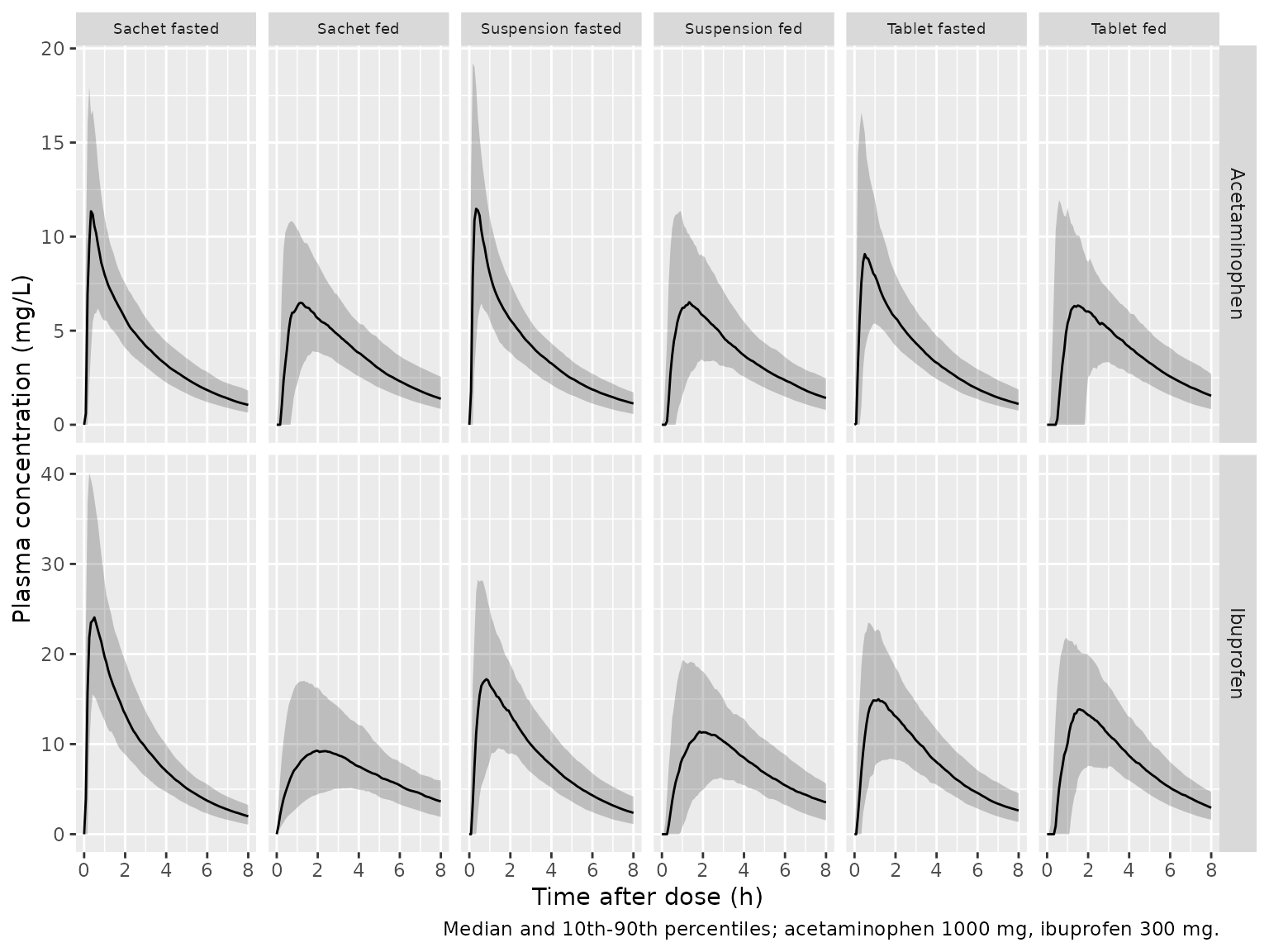
Replicate Table 4: simulated CMAX and TMAX
Table 4 reports medians and 10th / 90th percentiles of simulated
CMAX and TMAX after acetaminophen 1000 mg and
ibuprofen 300 mg. Two summaries of the virtual cohort are shown: the
noise-free individual prediction on a 5 min grid, and the observation
with residual error read off the paper’s sampling grid (Section 2.7).
The largest observation on a sparse grid overstates the true peak when
the residual error is large, which matters for ibuprofen (proportional
error 24% with 60% between-subject variability on its magnitude).
cmax_tmax <- function(d, value) {
  d |>
    group_by(drug, scenario, id) |>
    summarise(cmax = max(.data[[value]]), tmax = time[which.max(.data[[value]])], .groups = "drop") |>
    group_by(drug, scenario) |>
    summarise(
      cmax_med = median(cmax), cmax_p10 = quantile(cmax, 0.1), cmax_p90 = quantile(cmax, 0.9),
      tmax_med = median(tmax), tmax_p10 = quantile(tmax, 0.1), tmax_p90 = quantile(tmax, 0.9),
      .groups = "drop"
    )
}

on_clinical_grid <- sim_all |>
  filter(round(time * 60) %in% round(clinical_grid * 60))

sim_ipred <- cmax_tmax(sim_all, "Cc")
sim_obs <- cmax_tmax(on_clinical_grid, "sim")

fmt <- function(m, lo, hi, digits) {
  sprintf(paste0("%.", digits, "f (%.", digits, "f, %.", digits, "f)"), m, lo, hi)
}

table4_cmp <- table4 |>
  left_join(sim_ipred, by = c("drug", "scenario"), suffix = c("", "_ipred")) |>
  left_join(sim_obs, by = c("drug", "scenario"), suffix = c("", "_obs"))

table4_cmp |>
  transmute(
    drug, scenario,
    cmax_pub = fmt(cmax_med, cmax_p10, cmax_p90, 1),
    cmax_ipred = fmt(cmax_med_ipred, cmax_p10_ipred, cmax_p90_ipred, 1),
    cmax_obs = fmt(cmax_med_obs, cmax_p10_obs, cmax_p90_obs, 1),
    tmax_pub = fmt(tmax_med, tmax_p10, tmax_p90, 2),
    tmax_ipred = fmt(tmax_med_ipred, tmax_p10_ipred, tmax_p90_ipred, 2),
    tmax_obs = fmt(tmax_med_obs, tmax_p10_obs, tmax_p90_obs, 2)
  ) |>
  rename(
    "Drug" = drug,
    "Scenario" = scenario,
    "CMAX Table 4 (mg/L)" = cmax_pub,
    "CMAX simulated, IPRED (mg/L)" = cmax_ipred,
    "CMAX simulated, with RUV on sampling grid (mg/L)" = cmax_obs,
    "TMAX Table 4 (h)" = tmax_pub,
    "TMAX simulated, IPRED (h)" = tmax_ipred,
    "TMAX simulated, with RUV on sampling grid (h)" = tmax_obs
  ) |>
knitr::kable(caption = "Median (10th, 90th percentile) CMAX and TMAX: Table 4 of Morse 2022 versus the packaged models.")| Drug | Scenario | CMAX Table 4 (mg/L) | CMAX simulated, IPRED (mg/L) | CMAX simulated, with RUV on sampling grid (mg/L) | TMAX Table 4 (h) | TMAX simulated, IPRED (h) | TMAX simulated, with RUV on sampling grid (h) |
|---|---|---|---|---|---|---|---|
| Acetaminophen | Tablet fed | 10.9 (5.5, 19.8) | 7.8 (4.6, 14.5) | 7.7 (4.3, 15.5) | 0.88 (0.42, 1.82) | 1.50 (0.58, 3.50) | 1.50 (0.50, 3.00) |
| Acetaminophen | Suspension fed | 9.5 (4.8, 19.0) | 7.0 (4.0, 12.0) | 7.2 (4.2, 13.1) | 1.10 (0.50, 2.17) | 1.33 (0.66, 2.83) | 1.25 (0.75, 3.00) |
| Acetaminophen | Sachet fed | 9.9 (5.0, 19.4) | 7.2 (4.6, 12.5) | 7.5 (4.4, 13.1) | 1.03 (0.51, 1.99) | 1.25 (0.50, 2.76) | 1.25 (0.50, 3.00) |
| Acetaminophen | Tablet fasted | 12.8 (6.8, 24.2) | 10.2 (5.9, 17.8) | 10.8 (6.3, 18.6) | 0.61 (0.26, 1.24) | 0.58 (0.25, 1.26) | 0.75 (0.25, 1.25) |
| Acetaminophen | Suspension fasted | 15.1 (7.3, 31.2) | 12.8 (7.2, 19.8) | 13.3 (7.2, 20.3) | 0.31 (0.13, 0.72) | 0.33 (0.17, 0.75) | 0.50 (0.25, 1.00) |
| Acetaminophen | Sachet fasted | 14.4 (7.6, 28.6) | 12.8 (7.0, 19.4) | 12.7 (7.3, 20.0) | 0.35 (0.16, 0.86) | 0.42 (0.17, 0.75) | 0.50 (0.25, 1.00) |
| Ibuprofen | Tablet fed | 20.1 (10.3, 33.3) | 15.3 (8.6, 23.2) | 18.3 (8.8, 28.3) | 1.20 (0.68, 2.17) | 1.75 (0.83, 3.00) | 1.50 (1.00, 3.00) |
| Ibuprofen | Suspension fed | 16.2 (8.0, 30.3) | 12.7 (6.7, 20.9) | 14.1 (7.0, 25.6) | 1.55 (0.82, 2.63) | 2.12 (1.00, 3.92) | 2.00 (1.00, 3.00) |
| Ibuprofen | Sachet fed | 12.6 (6.1, 23.8) | 9.9 (5.4, 17.7) | 11.3 (6.0, 22.0) | 1.90 (1.12, 3.21) | 2.54 (1.17, 4.33) | 2.00 (0.98, 6.00) |
| Ibuprofen | Tablet fasted | 24.1 (13.3, 40.8) | 16.0 (8.9, 25.7) | 19.2 (10.4, 32.1) | 0.94 (0.48, 1.67) | 1.25 (0.58, 2.42) | 1.25 (0.50, 2.00) |
| Ibuprofen | Suspension fasted | 26.6 (14.8, 45.0) | 18.9 (10.4, 30.5) | 23.2 (12.1, 37.0) | 0.77 (0.40, 1.50) | 0.92 (0.42, 2.01) | 1.00 (0.50, 2.00) |
| Ibuprofen | Sachet fasted | 34.4 (20.8, 55.7) | 27.1 (17.5, 44.5) | 30.5 (18.4, 53.1) | 0.38 (0.19, 0.80) | 0.42 (0.17, 0.75) | 0.50 (0.25, 1.02) |
chk <- table4_cmp |>
  mutate(
    cmax_ratio_obs = cmax_med_obs / cmax_med,
    tmax_ratio_ipred = tmax_med_ipred / tmax_med
  )
knitr::kable(
  chk |>
    select(drug, scenario, cmax_ratio_obs, tmax_ratio_ipred) |>
    rename(
      "Drug" = drug,
      "Scenario" = scenario,
      "CMAX ratio, simulated with RUV / Table 4" = cmax_ratio_obs,
      "TMAX ratio, simulated IPRED / Table 4" = tmax_ratio_ipred
    ),
  digits = 2,
  caption = "Ratios of the simulated medians to the Table 4 medians."
)| Drug | Scenario | CMAX ratio, simulated with RUV / Table 4 | TMAX ratio, simulated IPRED / Table 4 |
|---|---|---|---|
| Acetaminophen | Tablet fed | 0.71 | 1.70 |
| Acetaminophen | Suspension fed | 0.76 | 1.21 |
| Acetaminophen | Sachet fed | 0.75 | 1.21 |
| Acetaminophen | Tablet fasted | 0.84 | 0.96 |
| Acetaminophen | Suspension fasted | 0.88 | 1.08 |
| Acetaminophen | Sachet fasted | 0.88 | 1.19 |
| Ibuprofen | Tablet fed | 0.91 | 1.46 |
| Ibuprofen | Suspension fed | 0.87 | 1.37 |
| Ibuprofen | Sachet fed | 0.90 | 1.34 |
| Ibuprofen | Tablet fasted | 0.80 | 1.33 |
| Ibuprofen | Suspension fasted | 0.87 | 1.19 |
| Ibuprofen | Sachet fasted | 0.89 | 1.10 |
# Medians over the 12 cells. The packaged models run about 15% below the
# Table 4 CMAX medians (see text); a mis-transcribed volume, bioavailability,
# dose or unit moves CMAX by a factor approaching 2 and leaves this band.
# TMAX: the fed scenarios run later than Table 4; a swapped fed-factor
# reference or a minutes-for-hours slip moves the median ratio far outside.
stopifnot(
  median(chk$cmax_ratio_obs) > 0.70,
  median(chk$cmax_ratio_obs) < 1.00,
  median(chk$tmax_ratio_ipred) > 0.85,
  median(chk$tmax_ratio_ipred) < 1.50
)
The simulated CMAX medians (with residual error, on the
sampling grid) are about 10-30% lower than Table 4, and the fed
TMAX medians are 20-70% later; the fasted acetaminophen
TMAX medians agree to within 20%. The packaged parameters
were not adjusted. Two observations from the paper itself suggest that
Table 4 does not follow directly from the printed parameters:
- Even for the typical individual (no random effects), the printed
parameters give an acetaminophen fasted-tablet
CMAXof about 11.0 mg/L and an ibuprofen fasted-tabletCMAXof about 17.6 mg/L, below the Table 4 medians of 12.8 and 24.1 mg/L. - Table 4’s upper percentiles exceed the observed concentrations in Supplementary Figures S3 and S4. The ibuprofen sachet 90th percentile is 55.7 mg/L, while no observed sachet concentration (fasted and fed pooled) exceeds about 38 mg/L; the fasted ibuprofen suspension median is 26.6 mg/L, about the largest observed suspension concentration. The simulated percentiles from the packaged models sit inside the observed ranges.
The ordering of the scenarios (fasted sachet and suspension fastest;
feeding lowering CMAX and delaying TMAX for
every formulation) is reproduced.
PKNCA validation
PKNCA on the noise-free individual predictions, grouped by drug and scenario. The paper reports no NCA of its own beyond Table 4, so the PKNCA medians are compared with the Table 4 medians.
sim_nca <- sim_all |>
  filter(!is.na(Cc)) |>
  select(id, time, Cc, drug, scenario)
sim_nca <- bind_rows(
  sim_nca,
  sim_nca |> distinct(id, drug, scenario) |> mutate(time = 0, Cc = 0)
) |>
  distinct(id, drug, scenario, time, .keep_all = TRUE) |>
  arrange(drug, scenario, id, time)

dose_nca <- bind_rows(
  events_apap |> filter(evid == 1) |> mutate(drug = "Acetaminophen"),
  events_ibu |> filter(evid == 1) |> mutate(drug = "Ibuprofen")
) |>
  select(id, time, amt, drug, scenario)

conc_obj <- PKNCA::PKNCAconc(sim_nca, Cc ~ time | drug + scenario + id)
dose_obj <- PKNCA::PKNCAdose(dose_nca, amt ~ time | drug + scenario + id)
intervals <- data.frame(
  start = 0, end = 12,
  cmax = TRUE, tmax = TRUE, auclast = TRUE
)
nca_res <- PKNCA::pk.nca(PKNCA::PKNCAdata(conc_obj, dose_obj, intervals = intervals))

reference <- table4 |>
  transmute(drug, scenario, cmax = cmax_med, tmax = tmax_med)

cmp <- nlmixr2lib::ncaComparisonTable(
  simulated = nca_res,
  reference = reference,
  by = c("drug", "scenario"),
  units = c(cmax = "mg/L", tmax = "h"),
  tolerance_pct = 20
)
knitr::kable(cmp, caption = "PKNCA medians of the noise-free simulations versus the Table 4 medians. * differs from the reference by more than 20%.")| NCA parameter | drug | scenario | Reference | Simulated | % diff |
|---|---|---|---|---|---|
| Cmax (mg/L) | Acetaminophen | Tablet fed | 10.9 | 7.78 | -28.6%* |
| Cmax (mg/L) | Acetaminophen | Suspension fed | 9.53 | 7.01 | -26.5%* |
| Cmax (mg/L) | Acetaminophen | Sachet fed | 9.91 | 7.22 | -27.1%* |
| Cmax (mg/L) | Acetaminophen | Tablet fasted | 12.8 | 10.2 | -20.3%* |
| Cmax (mg/L) | Acetaminophen | Suspension fasted | 15.1 | 12.8 | -14.9% |
| Cmax (mg/L) | Acetaminophen | Sachet fasted | 14.4 | 12.8 | -10.9% |
| Cmax (mg/L) | Ibuprofen | Tablet fed | 20.1 | 15.3 | -24.1%* |
| Cmax (mg/L) | Ibuprofen | Suspension fed | 16.2 | 12.7 | -21.7%* |
| Cmax (mg/L) | Ibuprofen | Sachet fed | 12.6 | 9.86 | -21.8%* |
| Cmax (mg/L) | Ibuprofen | Tablet fasted | 24.1 | 16 | -33.5%* |
| Cmax (mg/L) | Ibuprofen | Suspension fasted | 26.6 | 18.9 | -28.9%* |
| Cmax (mg/L) | Ibuprofen | Sachet fasted | 34.4 | 27.1 | -21.2%* |
| Tmax (h) | Acetaminophen | Tablet fed | 0.88 | 1.5 | +70.5%* |
| Tmax (h) | Acetaminophen | Suspension fed | 1.1 | 1.33 | +21.2%* |
| Tmax (h) | Acetaminophen | Sachet fed | 1.03 | 1.25 | +21.4%* |
| Tmax (h) | Acetaminophen | Tablet fasted | 0.61 | 0.583 | -4.4% |
| Tmax (h) | Acetaminophen | Suspension fasted | 0.31 | 0.333 | +7.5% |
| Tmax (h) | Acetaminophen | Sachet fasted | 0.35 | 0.417 | +19.0% |
| Tmax (h) | Ibuprofen | Tablet fed | 1.2 | 1.75 | +45.8%* |
| Tmax (h) | Ibuprofen | Suspension fed | 1.55 | 2.12 | +37.1%* |
| Tmax (h) | Ibuprofen | Sachet fed | 1.9 | 2.54 | +33.8%* |
| Tmax (h) | Ibuprofen | Tablet fasted | 0.94 | 1.25 | +33.0%* |
| Tmax (h) | Ibuprofen | Suspension fasted | 0.77 | 0.917 | +19.0% |
| Tmax (h) | Ibuprofen | Sachet fasted | 0.38 | 0.417 | +9.6% |
The starred rows are the CMAX and fed TMAX
differences discussed in the previous section. The noise-free
CMAX medians are lower than the residual-error summaries
above, because the largest of several noisy observations overstates the
true peak. Table 4’s footnote says CMAX and
TMAX were calculated from simulations; it does not say
whether residual error was included.
Total body composition: typical clearance and volume across weight
size_grid <- tidyr::crossing(WT = seq(50, 120, by = 5), SEXF = c(0L, 1L)) |>
  mutate(id = row_number(), HT = ifelse(SEXF == 1L, 163, 176), time = 0, amt = 0, evid = 0L, cmt = "central",
         FED = 0L, FORM_APAPIBU_SUSP = 0L, FORM_POWDER = 0L)
size_par <- bind_rows(
  rxode2::rxSolve(rxode2::zeroRe(mod_apap), size_grid, keep = c("WT", "SEXF"), returnType = "data.frame") |>
    mutate(drug = "Acetaminophen"),
  rxode2::rxSolve(rxode2::zeroRe(mod_ibu), size_grid, keep = c("WT", "SEXF"), returnType = "data.frame") |>
    mutate(drug = "Ibuprofen")
) |>
  select(drug, WT, SEXF, cl, vc) |>
  tidyr::pivot_longer(c(cl, vc), names_to = "parameter") |>
  mutate(parameter = ifelse(parameter == "cl", "CL (L/h)", "V1 (L)"), sex = ifelse(SEXF == 1, "female, 163 cm", "male, 176 cm"))
#> ℹ parameter labels from comments will be replaced by 'label()'
#> Warning: No sigma parameters in the model
#> ℹ omega/sigma items treated as zero: 'etalcl', 'etalvc', 'etalq', 'etalvp', 'etalfdepot', 'etaltabs', 'etaltlag', 'etaRUV'
#> Warning: multi-subject simulation without without 'omega'
#> ℹ parameter labels from comments will be replaced by 'label()'
#> Warning: No sigma parameters in the model
#> ℹ omega/sigma items treated as zero: 'etalcl', 'etalvc', 'etalq', 'etalvp', 'etalfdepot', 'etaltabs', 'etaltlag', 'etaRUV'
#> Warning: multi-subject simulation without without 'omega'

ggplot(size_par, aes(WT, value, colour = sex)) +
  geom_line() +
  facet_wrap(drug ~ parameter, scales = "free_y", nrow = 1) +
  labs(x = "Total body weight (kg)", y = "Typical value", colour = NULL) +
  theme(legend.position = "bottom")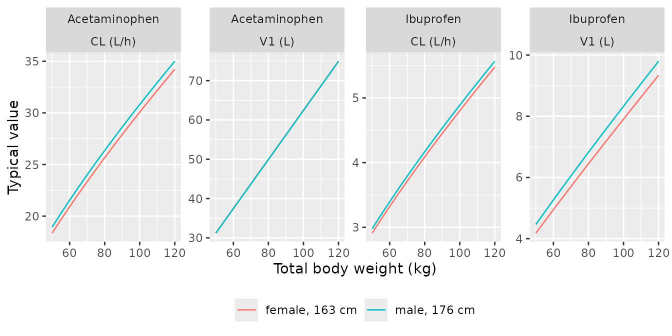
Pain-score simulation (Supplementary Table S4)
Morse 2022 simulated the time to a 2-point reduction in a 0-10 pain
score for a typical 70 kg individual, using the PK models above and the
acetaminophen + ibuprofen pharmacodynamic model of Hannam 2018
(Paediatr Anaesth 28:841-851, reproduced as Supplementary Table
S3). The pharmacodynamic model belongs to Hannam 2018 and is not part of
the packaged models; it is coded here only to check the absorption
parameters against Supplementary Table S4. Each drug is simulated alone
with an effect compartment and a sigmoid Emax model,
E = EMAX * Ce^HILL / (C50^HILL + Ce^HILL), and the
pain-score reduction is taken as 10 * E (a baseline of 10
is an assumption; the supplement does not state the baseline score).
# Hannam 2018 parameters (Supplementary Table S3) enter as data columns:
# tkeo = equilibration half-time (h), c50 (mg/L); EMAX 0.648 and HILL 1.48
# are shared by both drugs.
pd_layer <- function(mod) {
  mod |>
    rxode2::zeroRe() |>
    rxode2::model(d / dt(ce) <- log(2) / tkeo * (Cc - ce), append = TRUE) |>
    rxode2::model(pain_red <- 10 * 0.648 * ce^1.48 / (c50^1.48 + ce^1.48), append = TRUE)
}

time_to_2 <- function(mod, dose, tkeo, c50, params = NULL) {
  ev <- typical_events(dose, tgrid = seq(0, 3, by = 1 / 600)) |>
    filter(FED == 0L) |>
    mutate(tkeo = tkeo, c50 = c50)
  s <- rxode2::rxSolve(mod, ev, params = params, keep = "scenario", returnType = "data.frame")
  s |>
    group_by(scenario) |>
    summarise(minutes = 60 * time[which(pain_red >= 2)[1]], .groups = "drop")
}

pd_apap <- pd_layer(mod_apap)
#> ℹ parameter labels from comments will be replaced by 'label()'
#> Warning: No sigma parameters in the model
#> ℹ promote `tkeo` to population parameter with initial estimate 1
pd_ibu <- pd_layer(mod_ibu)
#> ℹ parameter labels from comments will be replaced by 'label()'
#> Warning: No sigma parameters in the model
#> ℹ promote `tkeo` to population parameter with initial estimate 1
no_lag <- c(ltlag = log(1e-6))

pain <- bind_rows(
  full_join(time_to_2(pd_apap, 1000, 0.34, 7.06) |> rename(with_lag = minutes),
    time_to_2(pd_apap, 1000, 0.34, 7.06, no_lag) |> rename(no_lag = minutes),
    by = "scenario"
  ) |> mutate(drug = "Acetaminophen"),
  full_join(time_to_2(pd_ibu, 300, 1.04, 3.95) |> rename(with_lag = minutes),
    time_to_2(pd_ibu, 300, 1.04, 3.95, no_lag) |> rename(no_lag = minutes),
    by = "scenario"
  ) |> mutate(drug = "Ibuprofen")
) |>
  left_join(
    tibble::tribble(
      ~drug, ~scenario, ~published,
      "Acetaminophen", "Tablet fasted", 21.8,
      "Acetaminophen", "Suspension fasted", 14.3,
      "Acetaminophen", "Sachet fasted", 15.0,
      "Ibuprofen", "Tablet fasted", 24.0,
      "Ibuprofen", "Suspension fasted", 24.8,
      "Ibuprofen", "Sachet fasted", 14.3
    ),
    by = c("drug", "scenario")
  )
#> ℹ omega/sigma items treated as zero: 'etalcl', 'etalvc', 'etalq', 'etalvp', 'etalfdepot', 'etaltabs', 'etaltlag', 'etaRUV'
#> Warning: multi-subject simulation without without 'omega'
#> ℹ omega/sigma items treated as zero: 'etalcl', 'etalvc', 'etalq', 'etalvp', 'etalfdepot', 'etaltabs', 'etaltlag', 'etaRUV'
#> Warning: multi-subject simulation without without 'omega'
#> ℹ omega/sigma items treated as zero: 'etalcl', 'etalvc', 'etalq', 'etalvp', 'etalfdepot', 'etaltabs', 'etaltlag', 'etaRUV'
#> Warning: multi-subject simulation without without 'omega'
#> ℹ omega/sigma items treated as zero: 'etalcl', 'etalvc', 'etalq', 'etalvp', 'etalfdepot', 'etaltabs', 'etaltlag', 'etaRUV'
#> Warning: multi-subject simulation without without 'omega'

pain |>
  select(drug, scenario, published, with_lag, no_lag) |>
  rename(
    "Drug" = drug,
    "Scenario" = scenario,
    "Table S4 (min)" = published,
    "Simulated, with lag time (min)" = with_lag,
    "Simulated, lag time removed (min)" = no_lag
  ) |>
knitr::kable(digits = 1, caption = "Time to a 2-point pain-score reduction for a typical 70 kg individual, fasted.")| Drug | Scenario | Table S4 (min) | Simulated, with lag time (min) | Simulated, lag time removed (min) |
|---|---|---|---|---|
| Acetaminophen | Sachet fasted | 15.0 | 19.6 | 15.2 |
| Acetaminophen | Suspension fasted | 14.3 | 18.2 | 14.2 |
| Acetaminophen | Tablet fasted | 21.8 | 27.0 | 21.7 |
| Ibuprofen | Sachet fasted | 14.3 | 15.7 | 12.1 |
| Ibuprofen | Suspension fasted | 24.8 | 27.2 | 20.6 |
| Ibuprofen | Tablet fasted | 24.0 | 31.2 | 24.5 |
# Deterministic typical-value checks: with the lag time every time is within
# 10 min of Supplementary Table S4; without it the acetaminophen times are
# within 1 min.
acet_no_lag <- pain |> filter(drug == "Acetaminophen")
stopifnot(
  all(abs(pain$with_lag - pain$published) < 10),
  all(abs(acet_no_lag$no_lag - acet_no_lag$published) < 1)
)
The acetaminophen times in Supplementary Table S4 are reproduced to within 0.2 min when the lag time is removed from the simulation, and are about 4-5 min later with the lag time. This suggests the published pain-score simulations omitted the absorption lag time for acetaminophen. The ibuprofen tablet is also reproduced (to within 0.5 min) without the lag time, but the ibuprofen suspension and sachet are not reproduced by either variant; the source of that difference could not be identified from the paper.
Assumptions and deviations
- Scaling of Q2 and V2. The paper gives the size and body-composition model for “clearance” and “volume of distribution” (Eqs. 1-5) and reports Q2 in L/h/70 kg and V2 in L/70 kg. The packaged models apply the clearance size factor (Ffat for CL, exponent 3/4) to Q2 and the volume size factor (Ffat for V, exponent 1) to V2, which is the usual convention of this group of authors.
-
NFM standard value.
NFM_STD = 56.1 + Ffat * (70 - 56.1)follows the paper’s definition (a 70 kg, 1.76 m male with FFM 56.1 kg). The packaged Janmahasatian equation gives 56.1 kg for that individual. -
Random effect on bioavailability. Eq. 6 states that
every random effect is exponential, so
F = F_pop * exp(eta). With the ibuprofenF = 0.941and a 5.1% PPV, about one subject in eight has an individualFslightly above 1. The paper does not report a logit or capped form. -
Residual error. Eq. 8 writes the proportional term
on the observation (
Obs); it is implemented on the model prediction, as NONMEM residual error models are. The additive and proportional SDs are combined as a sum of variances, as in Eq. 8, and both are scaled byexp(etaRUV). - Tablet strengths. The 500/150 mg and 325/97.5 mg film-coated tablets are modelled as one tablet formulation, as in the paper.
- Abstract values. The abstract gives the acetaminophen and ibuprofen central volumes as 43.5 and 10.5 L/70 kg; those are the Q2 values of Tables 2 and 3. The packaged models use the table values (V1 43.7 and 6.05 L/70 kg). The abstract and Discussion also give the acetaminophen bioavailability as 86% and 87%; Table 2 gives 0.859, which is used.
- Ibuprofen RUV PROP. Table 3 prints 24.0% with a bootstrap 95% CI of 19.9-22.1%, which excludes the estimate; the point estimate is used.
- Virtual cohort. Weight, height and sex are drawn to match Table 1 (no individual demographics are published). Ages are not needed by the models.
- Pain-score model. The Hannam 2018 pharmacodynamic layer is used only in this article, with an assumed baseline pain score of 10, to check Supplementary Table S4. It is not part of the packaged models.
- Errata. No correction notice for this article was found in Europe PMC (checked 2026-10-02).