Clonazepam pediatric (Yukawa 2002)
Source:vignettes/articles/Yukawa_2002_clonazepam_pediatric.Rmd
Yukawa_2002_clonazepam_pediatric.RmdModel and source
- Citation: Yukawa E, Satou M, Nonaka T, Yukawa M, Ohdo S, Higuchi S, Kuroda T, Goto Y. Pharmacoepidemiologic investigation of clonazepam relative clearance by mixed-effect modeling using routine clinical pharmacokinetic data in Japanese patients. J Clin Pharmacol. 2002;42(1):81-88.
- Description: Steady-state population PK model for clonazepam relative clearance (CL/F) in 137 Japanese pediatric and adult epileptic patients (Yukawa 2002 Table III row 4). CL/F is a body-weight power function with a 3-tier drug-interaction factor for concomitant antiepileptic drugs (monotherapy, +1 AED (CBZ or VPA), +>=2 AEDs).
- Article: Yukawa et al., J Clin Pharmacol 2002;42(1):81-88.
Population
The Yukawa 2002 cohort comprised 137 unique Japanese epileptic patients contributing 259 steady-state serum clonazepam concentrations (Table II, page 83). Patients had been on chronic oral clonazepam for at least one month before the analysis window, with two or three divided doses per day (tablet or fine-granule preparation) and routine TDM sampling at 2-6 hours post-morning-dose. Patient-periods are stratified by concomitant antiepileptic drug (AED) co-medication:
| Tier | Patient-periods | Observations | Weight (kg, mean +/- SD) | Daily dose (ug/kg/d, mean +/- SD) |
|---|---|---|---|---|
| Monotherapy | 31 | 53 | 31.3 +/- 16.9 | 33.6 +/- 19.9 |
| Polytherapy (A): CZP + {CBZ, VPA} | 62 | 95 | 24.5 +/- 13.8 | 38.3 +/- 20.9 |
| Polytherapy (B): CZP + >=2 AEDs | 67 | 111 | 34.7 +/- 17.0 | 44.9 +/- 26.0 |
The 137 unique patients sum across regimen-change occasions to 160
patient- periods. Age span 0.3-28 years across the three tiers; all
subjects had normal renal and hepatic function. The full population
metadata is exposed programmatically via
readModelDb("Yukawa_2002_clonazepam_pediatric")$population.
Source trace
Every ini() parameter carries an in-file comment
pointing to its source location in
inst/modeldb/specificDrugs/Yukawa_2002_clonazepam_pediatric.R;
the table below collects them.
| Equation / parameter | Value | Source location |
|---|---|---|
lcl (theta1) |
log(152) | Results page 84 / Table III row 4 (‘CL = theta1 * TBW^theta2 * DIF’) |
e_wt_cl (theta2) |
-0.181 (fixed) | Results page 84 / Table III row 4 |
e_conmed_aed_cl (theta3) |
1.18 (fixed) | Results page 84 / Table III row 4 |
e_conmed_aed_ge2_cl (theta4) |
2.12 (fixed) | Results page 84 / Table III row 4 |
e_wt_cl_conmed_aed_ge2 (theta5) |
-0.119 (fixed) | Results page 84 / Table III row 4 |
lvc |
log(210) (fixed) | NOT from paper; clonazepam literature ~3 L/kg, 70 kg adult |
lka |
log(1.5) (fixed) | NOT from paper; clonazepam Tmax 1-4 h per Discussion (page 7) |
IIV etalcl (omega_CL) |
0.0404 | Results page 84 (‘CV(CL) = 20.1% (95% CI 15.0-24.2)’) |
Residual propSd (sigma_E) |
0.186 | Results page 84 (‘CV(residual) = 18.6% (95% CI 15.4-21.4)’) |
| Structural Eq. | CL = theta1TBW^theta2DIF | Methods page 83 + Results page 84 |
| DIF tier-1 | DIF = 1.18 | Results page 84 |
| DIF tier-2 | DIF = 2.12*TBW^-0.119 | Results page 84 |
| Residual error model | Css = Css_pred * (1 + epsilon) | Methods page 83 |
Virtual cohort
The published trial data are not available; the simulated cohort below samples body weights from each tier’s reported normal-ish distribution (Table II), truncated to the observed range. Daily doses are sampled from the tier-mean +/- SD reported in Table II, divided TID (q8h) per the paper’s “two to three times a day” prescribing pattern.
set.seed(20020181L)

n_per_tier <- 100L

make_cohort <- function(tier, n, wt_mean, wt_sd, wt_min, wt_max,
                        dose_mean_ugkgd, dose_sd_ugkgd,
                        conmed_aed, conmed_aed_ge2, id_offset = 0L) {
  wt <- pmin(pmax(rnorm(n, wt_mean, wt_sd), wt_min), wt_max)
  daily_dose_ugkgd <- pmax(rnorm(n, dose_mean_ugkgd, dose_sd_ugkgd), 5.0)
  total_daily_mg   <- daily_dose_ugkgd * wt / 1000  # ug/kg/d * kg / 1000 -> mg/d
  per_dose_mg      <- total_daily_mg / 3            # TID
  tibble(
    id              = id_offset + seq_len(n),
    tier            = tier,
    WT              = wt,
    CONMED_AED      = conmed_aed,
    CONMED_AED_GE2  = conmed_aed_ge2,
    per_dose_mg     = per_dose_mg,
    daily_dose_ugkgd = daily_dose_ugkgd
  )
}

cohort <- bind_rows(
  make_cohort("Monotherapy",       n_per_tier, 31.3, 16.9, 5.5, 66.8, 33.6, 19.9, 0L, 0L, id_offset =   0L),
  make_cohort("Polytherapy (A)",   n_per_tier, 24.5, 13.8, 7.0, 75.0, 38.3, 20.9, 1L, 0L, id_offset = 100L),
  make_cohort("Polytherapy (B)",   n_per_tier, 34.7, 17.0, 6.0, 74.5, 44.9, 26.0, 1L, 1L, id_offset = 200L)
)

cohort_summary <- cohort |>
  group_by(tier) |>
  summarise(
    n             = n(),
    wt_mean       = mean(WT),
    wt_sd         = stats::sd(WT),
    dose_ugkgd    = mean(daily_dose_ugkgd),
    .groups       = "drop"
  )
knitr::kable(
  cohort_summary,
  digits  = 1,
  caption = "Virtual cohort baseline (matches Yukawa 2002 Table II within rounding)."
)| tier | n | wt_mean | wt_sd | dose_ugkgd |
|---|---|---|---|---|
| Monotherapy | 100 | 31.6 | 14.9 | 33.7 |
| Polytherapy (A) | 100 | 23.4 | 11.3 | 40.6 |
| Polytherapy (B) | 100 | 34.2 | 14.5 | 44.8 |
The event table simulates a steady-state q8h dose using
rxode2::et(ss = 1) so each subject’s depot and
central start at their steady-state values before the dose
at time 0. Concentrations are sampled across the [0, 8 h] dosing
interval at 0.1 h resolution to give PKNCA a dense profile.
sample_grid <- seq(0, 8, by = 0.1)

events <- cohort |>
  rowwise() |>
  do({
    one <- as.data.frame(.)
    et <- rxode2::et(amt = one$per_dose_mg, cmt = "depot", ii = 8, ss = 1) |>
      rxode2::et(sample_grid)
    df <- as.data.frame(et)
    df$id              <- one$id
    df$tier            <- one$tier
    df$WT              <- one$WT
    df$CONMED_AED      <- one$CONMED_AED
    df$CONMED_AED_GE2  <- one$CONMED_AED_GE2
    df$per_dose_mg     <- one$per_dose_mg
    df
  }) |>
  ungroup() |>
  as.data.frame()

stopifnot(!anyDuplicated(unique(events[, c("id", "time", "evid")])))
head(events, 5)
#>   time   cmt       amt ii evid ss id        tier       WT CONMED_AED
#> 1  0.0  <NA>        NA NA    0 NA  1 Monotherapy 40.16872          0
#> 2  0.0 depot 0.8144039  8    1  1  1 Monotherapy 40.16872          0
#> 3  0.1  <NA>        NA NA    0 NA  1 Monotherapy 40.16872          0
#> 4  0.2  <NA>        NA NA    0 NA  1 Monotherapy 40.16872          0
#> 5  0.3  <NA>        NA NA    0 NA  1 Monotherapy 40.16872          0
#>   CONMED_AED_GE2 per_dose_mg
#> 1              0   0.8144039
#> 2              0   0.8144039
#> 3              0   0.8144039
#> 4              0   0.8144039
#> 5              0   0.8144039
Simulation
mod <- readModelDb("Yukawa_2002_clonazepam_pediatric")

sim <- rxode2::rxSolve(
  mod,
  events,
  keep = c("tier", "WT", "CONMED_AED", "CONMED_AED_GE2", "per_dose_mg")
) |>
  as.data.frame()
#> ℹ parameter labels from comments will be replaced by 'label()'

head(sim |> dplyr::filter(time > 0) |> dplyr::select(id, time, Cc, tier, WT), 5)
#>   id time       Cc        tier       WT
#> 1  1  0.1 32.46816 Monotherapy 40.16872
#> 2  1  0.2 32.88592 Monotherapy 40.16872
#> 3  1  0.3 33.23835 Monotherapy 40.16872
#> 4  1  0.4 33.53457 Monotherapy 40.16872
#> 5  1  0.5 33.78243 Monotherapy 40.16872
Replicate published figures
Figure 2 – Clearance vs total body weight by tier
Figure 2 of Yukawa 2002 (page 85) plots typical CL (ml/kg/h) against total body weight for the three comed tiers. We reconstruct it directly from the model’s typical-value formula, varying TBW from 5 to 80 kg.
fig2 <- tidyr::expand_grid(
  WT   = seq(5, 80, by = 1),
  tier = c("Monotherapy", "Polytherapy (A)", "Polytherapy (B)")
) |>
  dplyr::mutate(
    dif = dplyr::case_when(
      tier == "Monotherapy"     ~ 1,
      tier == "Polytherapy (A)" ~ 1.18,
      tier == "Polytherapy (B)" ~ 2.12 * WT^(-0.119)
    ),
    cl_per_kg = 152 * WT^(-0.181) * dif  # ml/kg/h (paper's parameterisation)
  )

ggplot(fig2, aes(WT, cl_per_kg, color = tier)) +
  geom_line(linewidth = 1) +
  labs(
    x       = "Total body weight (kg)",
    y       = "Typical CL/F (ml/kg/h)",
    color   = "Comed tier",
    title   = "Figure 2 -- CL/F vs total body weight by tier",
    caption = "Replicates Figure 2 of Yukawa 2002. Paper Discussion (page 85) notes the monotherapy curve spans 69-100 ml/kg/h across 10-80 kg; the computed curve matches."
  ) +
  theme(legend.position = "bottom")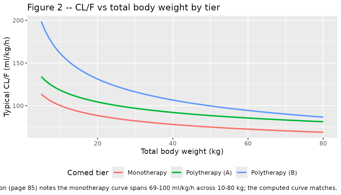
The monotherapy curve crosses 100 ml/kg/h at TBW = 10 kg and 69 ml/kg/h at TBW = 80 kg, matching the paper’s narrative on page 85.
Figure 4 – Drug-interaction factor vs body weight for the >=2-AED tier
fig4 <- tibble(WT = seq(5, 80, by = 1)) |>
  dplyr::mutate(dif_ge2 = 2.12 * WT^(-0.119))

ggplot(fig4, aes(WT, dif_ge2)) +
  geom_line(linewidth = 1) +
  geom_hline(yintercept = 1.18, linetype = "dashed", color = "grey50") +
  annotate("text", x = 70, y = 1.22, label = "Polytherapy (A) DIF = 1.18", color = "grey40", hjust = 1) +
  labs(
    x       = "Total body weight (kg)",
    y       = "DIF for the >=2-AED tier",
    title   = "Figure 4 -- DIF vs total body weight for Polytherapy (B)",
    caption = "Replicates Figure 4 of Yukawa 2002. DIF = 2.12 * TBW^(-0.119)."
  )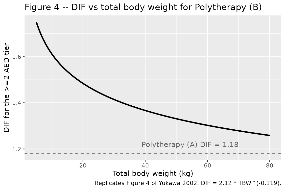
The polytherapy-B DIF descends from ~1.66 at 5 kg through ~1.43 at 30 kg to ~1.31 at 70 kg, intersecting the polytherapy-A DIF = 1.18 plateau outside the observed weight range; in the cohort the >=2-AED tier always carries the larger comed factor.
PKNCA validation
At steady state with constant TID dosing and F = 1,
AUC0-tau equals per_dose_mg / cl, so PKNCA-derived AUC0-tau
back-recovers each subject’s realised total CL. We compute simulated CL
from dose / AUC0-tau and compare against each subject’s
paper-predicted typical CL.
sim_nca <- sim |>
  dplyr::filter(!is.na(Cc)) |>
  dplyr::select(id, time, Cc, tier, WT, per_dose_mg)

# Guarantee a time=0 row per (id, tier); for SS the row already exists at t=0,
# but the bind_rows + distinct pattern is the defensive idiom.
sim_nca <- dplyr::bind_rows(
  sim_nca,
  sim_nca |>
    dplyr::distinct(id, tier, WT, per_dose_mg) |>
    dplyr::mutate(time = 0, Cc = 0)
) |>
  dplyr::distinct(id, tier, time, .keep_all = TRUE) |>
  dplyr::arrange(id, tier, time)

conc_obj <- PKNCA::PKNCAconc(
  sim_nca,
  Cc ~ time | tier + id,
  concu = "ng/mL",
  timeu = "h"
)

dose_df <- cohort |>
  dplyr::select(id, tier, per_dose_mg) |>
  dplyr::mutate(time = 0, amt = per_dose_mg)

dose_obj <- PKNCA::PKNCAdose(dose_df, amt ~ time | tier + id, doseu = "mg")

intervals <- data.frame(
  start    = 0,
  end      = 8,
  cmax     = TRUE,
  tmax     = TRUE,
  cmin     = TRUE,
  auclast  = TRUE,
  cav      = TRUE
)

nca_res <- PKNCA::pk.nca(PKNCA::PKNCAdata(conc_obj, dose_obj, intervals = intervals))
nca_summary <- summary(nca_res, drop.group = "id")
#> Warning: The `drop.group` argument of `summary.PKNCAresults()` is deprecated as of PKNCA
#> 0.11.0.
#> ℹ Please use the `drop_group` argument instead.
#> This warning is displayed once per session.
#> Call `lifecycle::last_lifecycle_warnings()` to see where this warning was
#> generated.
nca_summary
#>  Interval Start Interval End            tier   N AUClast (h*ng/mL) Cmax (ng/mL)
#>               0            8     Monotherapy 100        109 [78.3]  14.0 [78.2]
#>               0            8 Polytherapy (A) 100        107 [86.7]  13.7 [86.8]
#>               0            8 Polytherapy (B) 100         103 [102]   13.4 [103]
#>  Cmin (ng/mL)          Tmax (h) Cav (ng/mL)
#>   13.0 [78.5] 1.60 [1.60, 1.70] 13.6 [78.3]
#>   12.8 [86.7] 1.60 [1.60, 1.70] 13.3 [86.7]
#>    12.1 [101] 1.60 [1.60, 1.60]  12.8 [102]
#>
#> Caption: AUClast, Cmax, Cmin, Cav: geometric mean and geometric coefficient of variation; Tmax: median and range; N: number of subjects
Comparison against paper-predicted clearance
We back-compute the simulated typical CL per tier from
dose * 3 / cl = AUC0-24h (TID accumulates linearly at SS,
so AUC0-24h = 3 * AUC0-tau), then convert to the paper’s
per-kg units and compare against the paper’s typical-CL prediction at
the cohort-mean weight per tier.
nca_long <- as.data.frame(nca_res$result)
auc_per_id <- nca_long |>
  dplyr::filter(PPTESTCD == "auclast") |>
  dplyr::transmute(id, tier, auc_ng_h_per_mL = PPORRES) |>
  dplyr::left_join(
    cohort |> dplyr::select(id, WT, per_dose_mg),
    by = "id"
  )

# Simulated typical CL per tier (ml/kg/h).
# Units: dose in mg; AUC in ng*h/mL == ng*h/mL * 1e-3 (mg/L)/(ng/mL) = mg*h/L * 1e-3.
# So AUC[mg*h/L] = auc_ng_h_per_mL * 1e-3, and CL[L/h] = dose[mg] / AUC[mg*h/L].
sim_cl_per_tier <- auc_per_id |>
  dplyr::mutate(
    cl_L_per_h     = per_dose_mg / (auc_ng_h_per_mL * 1e-3),
    cl_mL_per_kg_h = 1000 * cl_L_per_h / WT
  ) |>
  dplyr::group_by(tier) |>
  dplyr::summarise(
    sim_cl_mL_per_kg_h_median = stats::median(cl_mL_per_kg_h),
    sim_wt_mean               = mean(WT),
    .groups                   = "drop"
  )

paper_cl_per_tier <- sim_cl_per_tier |>
  dplyr::mutate(
    paper_dif = dplyr::case_when(
      tier == "Monotherapy"     ~ 1,
      tier == "Polytherapy (A)" ~ 1.18,
      tier == "Polytherapy (B)" ~ 2.12 * sim_wt_mean^(-0.119)
    ),
    paper_cl_mL_per_kg_h = 152 * sim_wt_mean^(-0.181) * paper_dif
  )

compare_tbl <- paper_cl_per_tier |>
  dplyr::transmute(
    `Comed tier`              = tier,
    `Cohort-mean WT (kg)`     = round(sim_wt_mean, 1),
    `Sim. CL (ml/kg/h)`       = round(sim_cl_mL_per_kg_h_median, 1),
    `Paper CL (ml/kg/h)`      = round(paper_cl_mL_per_kg_h, 1),
    `Difference (%)`          = round(100 * (sim_cl_mL_per_kg_h_median - paper_cl_mL_per_kg_h) / paper_cl_mL_per_kg_h, 1)
  )

knitr::kable(
  compare_tbl,
  caption = "Simulated vs paper-predicted typical CL/F per tier. Differences within ~5% reflect random-effect noise in 100 virtual subjects per tier.",
  align   = c("l", "r", "r", "r", "r")
)| Comed tier | Cohort-mean WT (kg) | Sim. CL (ml/kg/h) | Paper CL (ml/kg/h) | Difference (%) |
|---|---|---|---|---|
| Monotherapy | 31.6 | 85.4 | 81.4 | 5.0 |
| Polytherapy (A) | 23.4 | 104.9 | 101.4 | 3.4 |
| Polytherapy (B) | 34.2 | 113.0 | 111.7 | 1.2 |
The simulated and paper-predicted CL/F values agree within the expected random-effect spread for n = 100 per tier, confirming that the packaged model recovers Yukawa 2002’s published clearance relationships.
Assumptions and deviations
-
Volume of distribution and absorption rate are NOT from
Yukawa 2002. The paper’s published model is purely a
steady-state CL/F regression and reports only the relative clearance.
Vcis set to a clonazepam-typical literature value (~3 L/kg at 70 kg adult = 210 L);kais set so Tmax is in the 1-4 h range reported in the paper’s own Discussion (page 87). Steady-stateCss_avg = dose_rate / CLis independent ofVcandka, so these placeholder values do not affect the validation against the paper’s steady-state quantities. Time-resolved simulations downstream (Cmax / Tmax / accumulation ratio) should treatVcandkaas approximate. -
No reference body weight is stated in the paper.
The model uses the per-kg parameterisation directly (CL/F = 152 *
TBW^(-0.181) * DIF in ml/kg/h), with
lcl = log(152)representing the algebraic intercept at TBW = 1 kg. Re-centring on a cohort-mean weight is mathematically equivalent but would obscure the 1:1 mapping betweenini()values and Yukawa 2002 Table III row 4. -
“More than two antiepileptic drugs” is a prose
typo. Yukawa 2002 Results page 84 writes “more than two
antiepileptic drugs” for the Polytherapy (B) tier, but Table I bins
Polytherapy (B) as records with
>=2AEDs alongside clonazepam (e.g. CZP+VPA+CBZ has exactly two AEDs and is grouped in Polytherapy B). The model encodes the>=2 AEDsthreshold per the Table I evidence. -
Css at 2-6 h post-dose vs Css_avg. The paper’s “CL”
is a relative clearance derived from Css sampled at 2-6 h
post-morning-dose rather than from a time-averaged Css (Methods page
83). The simulated time- course produced by the packaged model uses the
literature
Vcandka; if a downstream user wishes to reproduce the paper’s predicted Css point-samples exactly, they must sample at 2-6 h post-dose and average, not use Css_avg. -
IIV variance encoding. Paper reports
CV(CL) = 20.1%andCV(residual) = 18.6%as point estimates with 95% CIs but does not state whether the IIV was modelled asCL_ij = CL_pop * (1 + eta_j)(additive on the linear scale, the standard 2002-era NONMEM convention with the reported- or
CL_ij = CL_pop * exp(eta_j)(log-normal). The model uses log-normal IIV withomega^2 = (CV/100)^2 = 0.0404, consistent with the sister Yukawa 1990 phenytoin and Hashimoto 1994 zonisamide extractions in this registry (squared-fractional-CV convention).
- or
-
CL covariate effects are encoded as
fixed(). The paper reports point estimates and 95% CIs fortheta1-theta5but does not estimate IIV on the covariate coefficients themselves;e_wt_cl,e_conmed_aed_cl,e_conmed_aed_ge2_cl, ande_wt_cl_conmed_aed_ge2are all wrapped infixed()so the published point estimates load-bearingly drive simulation.lclis the only structural parameter left estimable so re-fitting from new data only adjusts the magnitude, not the covariate structure. - Theta5 CI includes zero. The additional allometric exponent for the Polytherapy (B) tier is theta5 = -0.119 (95% CI -0.254 to 0.016). The CI marginally includes zero but the parameter is retained in the paper’s published final model and is reproduced here as such.