Phenobarbital (Stoschus 2025)
Source:vignettes/articles/Stoschus_2025_phenobarbital.Rmd
Stoschus_2025_phenobarbital.RmdModel and source
- Citation: Stoschus M, Schmidbauer ML, Starp J, Kunst S, Gakis G, Paal M, Vogeser M, Scharf-Janssen C, Liebchen U, Dimitriadis K. Optimizing phenobarbital dosing in critically ill patients with refractory and superrefractory status epilepticus using a population pharmacokinetic model. Epilepsia. 2025;66(10):3757-3768. doi:10.1111/epi.18517.
- Description: One-compartment population PK model for oral and intravenous phenobarbital in critically ill adults with refractory and superrefractory status epilepticus (Stoschus 2025), with first-order absorption (ka fixed at 1.9 /h from Viswanathan 1979 because the therapeutic-drug-monitoring samples were taken after the absorption phase), estimated oral bioavailability F = 0.96, and ideal body weight entering as allometric scaling on both volume of distribution (exponent 1) and clearance (exponent 0.75), centered on the cohort median IBW of 68.8 kg. Interindividual variability is carried on V and CL, interoccasion variability on CL across consecutive TDM sampling intervals, with a proportional residual-error model.
- Article: https://doi.org/10.1111/epi.18517
Stoschus 2025 developed a population pharmacokinetic model for phenobarbital in critically ill adults treated for refractory (RSE) and superrefractory (SRSE) status epilepticus, and used it to derive ideal-body-weight-based loading and maintenance dosing recommendations for a 12-h dosing schedule.
The structural model is one compartment with first-order absorption and first-order elimination. The absorption rate constant could not be estimated because most therapeutic drug monitoring (TDM) samples were drawn after the absorption phase, so it was fixed to a literature value. Ideal body weight (IBW) was the only covariate retained, entering as classical allometric scaling on both volume of distribution and clearance.
mod <- readModelDb("Stoschus_2025_phenobarbital")
ui <- rxode2::rxode(mod)
#> Warning: some etas defaulted to non-mu referenced, possible parsing error: etaiov_cl_1, etaiov_cl_2, etaiov_cl_3, etaiov_cl_4, etaiov_cl_5, etaiov_cl_6, etaiov_cl_7, etaiov_cl_8
#> as a work-around try putting the mu-referenced expression on a simple line
Population
The model was fit to 301 TDM samples from 37 adults treated between 2015 and 2024 at a single German neurointensive care unit (Stoschus 2025 Table 1). Thirty-five patients (95%) had superrefractory status epilepticus and two (5%) refractory status epilepticus; the median Status Epilepticus Severity Score was 5. Thirteen patients (35%) were female and the median age was 63 years (5th-95th percentile 24-83). Median total body weight was 78.5 kg and median ideal body weight 68.8 kg – the latter is the reference for the allometric terms. Renal function was largely preserved (median estimated glomerular filtration rate 102 mL/min, median serum creatinine 0.7 mg/dL), with three patients (8%) on renal replacement therapy.
Patients received guideline-directed loading doses of 10-20 mg/kg and maintenance doses of 1-4 mg/kg over a median treatment duration of 16 days (median administered dose 200 mg). Of 1242 doses, 824 (66%) were oral – tablets dispersed in water and given via gastric tube – and 418 (34%) were intravenous 5-min infusions. The median observed phenobarbital concentration was 32.8 mg/L, with a median of 6 TDM samples per patient.
str(ui$population)
#> List of 13
#>  $ species       : chr "human"
#>  $ n_subjects    : int 37
#>  $ n_studies     : int 1
#>  $ age_range     : chr "24.0-83.0 years (5th-95th percentile); all patients >= 18 years by inclusion criterion"
#>  $ age_median    : chr "63.0 years"
#>  $ weight_range  : chr "51.7-93.3 kg total body weight (5th-95th percentile)"
#>  $ weight_median : chr "78.5 kg total body weight; 68.8 kg ideal body weight (the allometric-scaling reference)"
#>  $ sex_female_pct: num 35.1
#>  $ race_ethnicity: chr "Not reported."
#>  $ disease_state : chr "Refractory (2 patients, 5%) and superrefractory (35 patients, 95%) status epilepticus in a neurointensive care "| __truncated__
#>  $ dose_range    : chr "Guideline-directed phenobarbital: loading doses 10-20 mg/kg and maintenance doses 1-4 mg/kg, median administere"| __truncated__
#>  $ regions       : chr "Germany (single center: LMU University Hospital, Munich)."
#>  $ notes         : chr "Retrospective single-center cohort of patients treated 2015-2024, contributing 301 therapeutic-drug-monitoring "| __truncated__
Source trace
Every ini() entry carries an in-file comment naming its
origin in
inst/modeldb/specificDrugs/Stoschus_2025_phenobarbital.R.
The table collects them for review.
| Equation / parameter | Value | Source location |
|---|---|---|
lfdepot (F) |
0.96 | Table 2, row F (RSE 3.95%; 95% CI 0.85-0.99) |
lka (ka, fixed) |
1.9 /h | Table 2, row k a, h-1 with footnote “ka was fixed
according to literature values”; Methods 2.2 |
lvc (V) |
34.3 L | Table 2, row V, L (RSE 12.7%; 95% CI 26.81-43.89) |
lcl (CL) |
0.38 L/h | Table 2, row CL, L/h (RSE 7.81%; 95% CI 0.32-0.44) |
e_ibw_vc (fixed) |
1 | Results 3.2, Equation 1:
V_i = V * (IBW_i / medIBW)^1
|
e_ibw_cl (fixed) |
0.75 | Results 3.2, Equation 2:
CL_i = CL * (IBW_i / medIBW)^0.75
|
reference medIBW
|
68.8 kg | Table 1, row “Ideal body weight, kg” (cohort median) |
etalvc |
0.50799 | Table 2 IIV row V: SD 0.71, CV 81.36%;
omega^2 = log(1 + 0.8136^2)
|
etalcl |
0.157914 | Table 2 IIV row CL: SD 0.4, CV 41.36%;
omega^2 = log(1 + 0.4136^2)
|
etaiov_cl_1..8 |
0.127331 | Table 2 IOV row CL: SD 0.36, CV 36.85%;
omega^2 = log(1 + 0.3685^2)
|
propSd |
0.082 | Table 2, row Proportional (RSE 7.76%; 95% CI
0.071-0.096) |
| one-compartment, first-order absorption and elimination | n/a | Methods 2.2; Results 3.2 |
| IIV on V and CL, IOV on CL, proportional RUV | n/a | Results 3.2, first paragraph |
The two structural equations are printed in the article as images;
the exponents were read from the PDF text layer as ^1 on V
(Equation 1) and ^.75 on CL (Equation 2).
Variance scale
Table 2 reports interindividual and interoccasion variability as an SD (rounded to two significant figures) alongside a CV% (four significant figures). Methods 2.2 states that a lognormal distribution was assumed. Round-tripping each row through the lognormal relation confirms the SD column is the omega on the log scale, so the variances used here are back-solved from the more precise CV%.
tibble::tibble(
  parameter = c("IIV V", "IIV CL", "IOV CL"),
  cv_pct    = c(81.36, 41.36, 36.85),
  sd_printed = c(0.71, 0.40, 0.36)
) |>
  mutate(
    omega2       = log(1 + (cv_pct / 100)^2),
    sd_backsolved = sqrt(omega2),
    cv_roundtrip = 100 * sqrt(exp(sd_printed^2) - 1)
  ) |>
  knitr::kable(digits = 4, caption =
"The printed SD reproduces the printed CV% and vice versa, confirming the lognormal log-scale reading.")| parameter | cv_pct | sd_printed | omega2 | sd_backsolved | cv_roundtrip |
|---|---|---|---|---|---|
| IIV V | 81.36 | 0.71 | 0.5080 | 0.7127 | 80.9626 |
| IIV CL | 41.36 | 0.40 | 0.1579 | 0.3974 | 41.6546 |
| IOV CL | 36.85 | 0.36 | 0.1273 | 0.3568 | 37.1985 |
Typical-value checks
Two quantities are fixed by the structural parameters and can be checked in closed form before any simulation.
The paper states an elimination half-life of 62.6 h, “derived from our estimated population-specific parameters” (Methods 2.3), which it used to justify assessing steady-state trough concentrations at t = 336 h.
V  <- 34.3
CL <- 0.38
c(published_h = 62.6, closed_form_h = log(2) * V / CL)
#>   published_h closed_form_h
#>      62.60000      62.56565
Results 3.2 also reports the weight-normalised typical values obtained when dividing by the cohort median total body weight of 78.5 kg.
c(V_L_per_kg_paper = 0.44, V_L_per_kg_model = V / 78.5,
  CL_L_h_kg_paper = 0.0048, CL_L_h_kg_model = CL / 78.5)
#> V_L_per_kg_paper V_L_per_kg_model  CL_L_h_kg_paper  CL_L_h_kg_model
#>      0.440000000      0.436942675      0.004800000      0.004840764
Virtual cohort and simulation
Original patient data are not public. Simulations below use virtual cohorts whose ideal body weights are the discrete values the paper simulated (55-80 kg in 5-kg steps), all inside the observed cohort range of 52.4-82.4 kg.
Occasions follow the paper’s definition – the interval between
consecutive TDM samples, cohort median 48 h – so the OCC
column advances every 48 h and is capped at the eight occasions the
model file encodes.
occ_of <- function(time) pmin(floor(time / 48) + 1, 8)

# Build one 12-h-schedule regimen: loading dose at t = 0, maintenance doses
# every 12 h thereafter, observed on `obs_times`.
regimen <- function(ld, md, route, ibw, obs_times, last_dose = 324) {
  cmt <- if (identical(route, "IV")) "central" else "depot"
  ev <- rxode2::et(amt = ld, cmt = cmt, time = 0)
  if (md > 0) {
    for (tt in seq(12, last_dose, by = 12)) {
      ev <- rxode2::et(ev, amt = md, cmt = cmt, time = tt)
    }
  }
  ev <- rxode2::et(ev, obs_times, cmt = "central")
  d <- as.data.frame(ev)
  d$IBW <- ibw
  d$OCC <- occ_of(d$time)
  d
}

# Solve a cohort. The seed is set immediately before every rxSolve so that
# runs sharing a seed and an event-table shape draw the *same* subjects --
# common random numbers, which is what makes dose grids comparable.
solve_cohort <- function(events, n, seed) {
  set.seed(seed)
  as.data.frame(rxode2::rxSolve(ui, events, nSub = n, returnType = "data.frame"))
}
Instrument check: are the published omegas actually realised?
Before using the cohort to judge the model, confirm the simulated cohort reproduces the parameters that were put into it. A validation built on a mis-drawn cohort measures nothing.
chk <- solve_cohort(regimen(1000, 0, "IV", 68.8, 12), n = 2000L, seed = 11L) |>
  filter(time == 12)

tibble::tibble(
  quantity = c("median V (L)", "median CL (L/h)", "sd(log V)", "sd(log CL)"),
  simulated = c(median(chk$vc), median(chk$cl), sd(log(chk$vc)), sd(log(chk$cl))),
  expected  = c(34.3, 0.38, sqrt(0.50799), sqrt(0.157914 + 0.127331))
) |>
  mutate(pct_diff = 100 * (simulated - expected) / expected) |>
  knitr::kable(digits = 4, caption =
"Simulated cohort reproduces the published typical values and the IIV (V) and IIV+IOV (CL) log-scale spreads.")| quantity | simulated | expected | pct_diff |
|---|---|---|---|
| median V (L) | 34.4200 | 34.3000 | 0.3498 |
| median CL (L/h) | 0.3840 | 0.3800 | 1.0446 |
| sd(log V) | 0.7012 | 0.7127 | -1.6155 |
| sd(log CL) | 0.5349 | 0.5341 | 0.1457 |
The clearance spread combines the interindividual and interoccasion terms, because at any single time point a subject carries one IIV draw and one occasion’s IOV draw.
Replicating Figure 2
Figure 2 of Stoschus 2025 shows concentration-time profiles at IBW 70 kg for a 12-h schedule with the optimal loading dose of 1100 mg and maintenance dose of 150 mg, across the four combinations of loading and maintenance route, with the median, the 50% prediction interval, and the 18-40 mg/L target band.
obs_grid <- sort(unique(c(seq(0, 336, by = 2), 12, 336)))

fig2 <- bind_rows(lapply(
  list(c("IV", "IV"), c("IV", "PO"), c("PO", "IV"), c("PO", "PO")),
  function(rr) {
    ld_route <- rr[1]; md_route <- rr[2]
    # Loading and maintenance routes can differ, so build the two dose blocks
    # separately and bind them.
    cmt_ld <- if (ld_route == "IV") "central" else "depot"
    cmt_md <- if (md_route == "IV") "central" else "depot"
    ev <- rxode2::et(amt = 1100, cmt = cmt_ld, time = 0)
    for (tt in seq(12, 324, by = 12)) ev <- rxode2::et(ev, amt = 150, cmt = cmt_md, time = tt)
    ev <- rxode2::et(ev, obs_grid, cmt = "central")
    d <- as.data.frame(ev); d$IBW <- 70; d$OCC <- occ_of(d$time)
    solve_cohort(d, n = 200L, seed = 303L) |>
      mutate(arm = paste0(ld_route, " load / ", md_route, " maint."))
  }
))

fig2 |>
  group_by(arm, time) |>
  summarise(Q25 = quantile(Cc, 0.25), Q50 = median(Cc), Q75 = quantile(Cc, 0.75),
            .groups = "drop") |>
  ggplot(aes(time, Q50)) +
  geom_ribbon(aes(ymin = Q25, ymax = Q75), alpha = 0.3, fill = "steelblue") +
  geom_line(linewidth = 0.6) +
  geom_hline(yintercept = c(18, 40), linetype = "dotted", colour = "red") +
  facet_wrap(~arm) +
  labs(x = "Time (h)", y = "Phenobarbital concentration (mg/L)",
       caption = paste("Replicates Figure 2 of Stoschus 2025: IBW 70 kg, loading dose 1100 mg,",
                       "maintenance dose 150 mg every 12 h. Line = median,",
                       "band = 50% prediction interval, dotted = 18-40 mg/L target range."))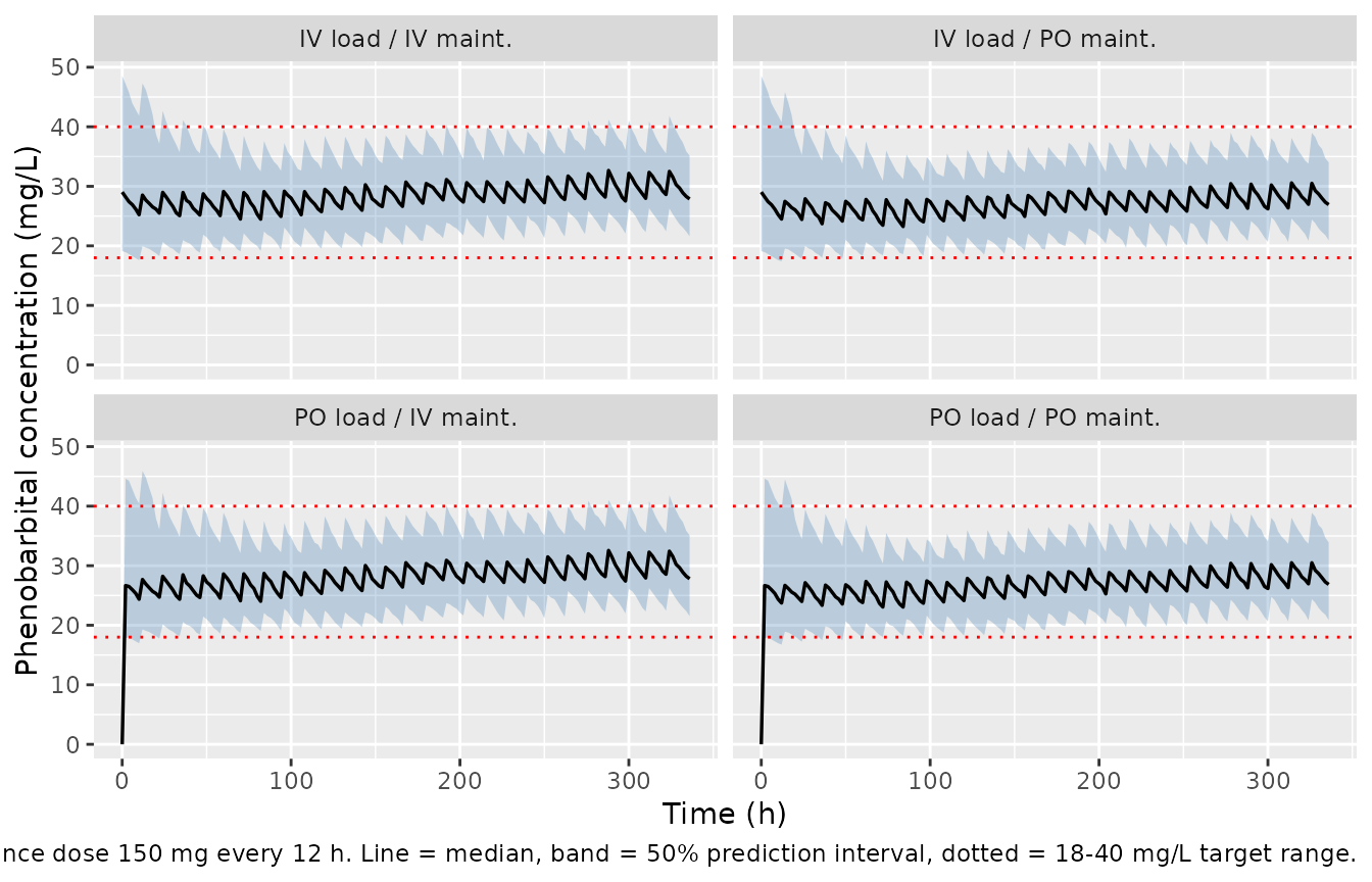
As the paper reports, the intravenous and oral profiles are nearly indistinguishable – a direct consequence of the 96% oral bioavailability.
fig2 |>
  filter(time == 336) |>
  group_by(arm) |>
  summarise(median_Cmin = median(Cc), .groups = "drop") |>
  knitr::kable(digits = 2, caption =
"Trough at t = 336 h by route combination; oral and intravenous agree closely.")| arm | median_Cmin |
|---|---|
| IV load / IV maint. | 27.88 |
| IV load / PO maint. | 26.93 |
| PO load / IV maint. | 27.82 |
| PO load / PO maint. | 26.87 |
PKNCA validation
NCA is run on a typical-value single-dose profile, where each
parameter has an exact closed-form counterpart. Using
zeroRe() matters here: with an 81% CV on volume the
population mean profile is not the typical-value profile, so a
cohort median would not be comparable to a closed-form identity.
ui_typ <- rxode2::zeroRe(ui)
#> Warning: some etas defaulted to non-mu referenced, possible parsing error: etaiov_cl_1, etaiov_cl_2, etaiov_cl_3, etaiov_cl_4, etaiov_cl_5, etaiov_cl_6, etaiov_cl_7, etaiov_cl_8
#> as a work-around try putting the mu-referenced expression on a simple line

nca_events <- regimen(1000, 0, "IV", 68.8, obs_times = sort(unique(
  c(seq(0, 24, by = 0.25), seq(24, 720, by = 2))
)))
set.seed(404L)
sim_nca_raw <- as.data.frame(
  rxode2::rxSolve(ui_typ, nca_events, returnType = "data.frame")
)
#> ℹ omega/sigma items treated as zero: 'etalvc', 'etalcl', 'etaiov_cl_1', 'etaiov_cl_2', 'etaiov_cl_3', 'etaiov_cl_4', 'etaiov_cl_5', 'etaiov_cl_6', 'etaiov_cl_7', 'etaiov_cl_8'
if (is.null(sim_nca_raw$id)) sim_nca_raw$id <- 1L

sim_nca <- sim_nca_raw |>
  filter(!is.na(Cc)) |>
  mutate(treatment = "1000 mg IV, typical value") |>
  select(id, time, Cc, treatment)

# Guarantee a time-zero anchor for AUC.
sim_nca <- bind_rows(
  sim_nca,
  sim_nca |> distinct(id, treatment) |> mutate(time = 0, Cc = 0)
) |>
  distinct(id, treatment, time, .keep_all = TRUE) |>
  arrange(id, treatment, time)

conc_obj <- PKNCA::PKNCAconc(sim_nca, Cc ~ time | treatment + id)

dose_df <- data.frame(id = 1L, time = 0, amt = 1000,
                      treatment = "1000 mg IV, typical value")
dose_obj <- PKNCA::PKNCAdose(dose_df, amt ~ time | treatment + id)

nca_res <- PKNCA::pk.nca(PKNCA::PKNCAdata(
  conc_obj, dose_obj,
  intervals = data.frame(start = 0, end = Inf,
                         cmax = TRUE, tmax = TRUE,
                         aucinf.obs = TRUE, half.life = TRUE)
))
Comparison against published and closed-form values
The paper reports one NCA-comparable quantity directly, the 62.6 h elimination half-life. The remaining rows are exact closed-form identities for a one-compartment intravenous bolus at the reference IBW, which gate the NCA machinery as well as the model: an error in the dosing route, the observation grid, or the PKNCA setup breaks the AUC identity immediately.
published <- tibble::tribble(
  ~treatment,                  ~cmax,   ~tmax, ~aucinf.obs, ~half.life,
  "1000 mg IV, typical value", 1000 / V, 0,     1000 / CL,   62.6
)

nlmixr2lib::ncaComparisonTable(
  simulated = nca_res,
  reference = published,
  by        = "treatment",
  units     = c(cmax = "mg/L", aucinf.obs = "mg*h/L", tmax = "h", half.life = "h"),
  tolerance_pct = 20
) |>
  knitr::kable(caption = paste(
    "Simulated vs reference NCA. half.life is the published 62.6 h;",
    "cmax = dose/V, aucinf.obs = dose/CL are closed-form identities.",
"* marks a >20% difference."))| NCA parameter | treatment | Reference | Simulated | % diff |
|---|---|---|---|---|
| Cmax (mg/L) | 1000 mg IV, typical value | 29.2 | 29.2 | +0.0% |
| Tmax (h) | 1000 mg IV, typical value | 0 | 0 | — |
| AUC0-∞ (obs) (mg*h/L) | 1000 mg IV, typical value | 2630 | 2630 | -0.0% |
| t½ (h) | 1000 mg IV, typical value | 62.6 | 62.6 | -0.1% |
The AUC identity AUC(0-inf) = dose / CL is the strongest
single check in this vignette: it simultaneously gates the ODE, the dose
encoding, the observation window, and PKNCA’s settings.
Replicating Table 3: optimal 12-h dosing
Table 3 of Stoschus 2025 gives, for each IBW from 55 to 80 kg, the loading and maintenance doses maximising the probability that the trough concentration falls in 18-40 mg/L. Loading doses were selected on the trough at t = 12 h and maintenance doses on the trough at t = 336 h, with the optimal loading dose applied first.
Because the model is linear in dose and the loading-dose trough involves a single dose, the whole 100-2500 mg loading grid can be evaluated exactly from one unit-dose solve per IBW and route – the same subjects are used at every dose, which removes the Monte Carlo noise that would otherwise dominate the comparison between adjacent doses.
u <- solve_cohort(regimen(1, 0, "IV", 70, 12), n = 200L, seed = 505L) |> filter(time == 12)
m <- solve_cohort(regimen(1100, 0, "IV", 70, 12), n = 200L, seed = 505L) |> filter(time == 12)
c(max_relative_error = max(abs(1100 * u$Cc - m$Cc) / m$Cc))
#> max_relative_error
#>       7.300765e-07
Dose-proportionality holds to machine precision, so the scaling is exact rather than an approximation.
IBWS <- seq(55, 80, by = 5)
in_target <- function(x) mean(x >= 18 & x <= 40)
load_grid <- seq(100, 2500, by = 100)

loading_published <- tibble::tibble(
  IBW = rep(IBWS, each = 2),
  route = rep(c("IV", "PO"), times = 6),
  dose_paper = c(1000, 900, 1000, 1000, 1000, 1000, 1100, 1100, 1300, 1300, 1300, 1300)
)

loading <- bind_rows(lapply(IBWS, function(ib) {
  bind_rows(lapply(c("IV", "PO"), function(rt) {
    unit <- solve_cohort(regimen(1, 0, rt, ib, 12), n = 200L, seed = 606L) |>
      filter(time == 12)
    p <- vapply(load_grid, function(D) in_target(D * unit$Cc), numeric(1))
    dp <- loading_published$dose_paper[loading_published$IBW == ib &
                                         loading_published$route == rt]
    tibble::tibble(IBW = ib, route = rt,
                   dose_model = load_grid[which.max(p)], pta = max(p),
                   dose_paper = dp, pta_at_paper = in_target(dp * unit$Cc))
  }))
}))

loading |>
  mutate(`PTA at model optimum (%)` = round(100 * pta, 1),
         `PTA at Table 3 dose (%)`  = round(100 * pta_at_paper, 1),
         `PTA loss (pp)` = round(100 * (pta - pta_at_paper), 1)) |>
  select(IBW, route, `Model optimum (mg)` = dose_model,
         `Table 3 (mg)` = dose_paper,
         `PTA at model optimum (%)`, `PTA at Table 3 dose (%)`, `PTA loss (pp)`) |>
  knitr::kable(caption = paste(
    "Loading doses: model optimum vs Stoschus 2025 Table 3. The last column is a",
    "paired comparison on identical subjects, so it isolates the dose choice from",
"Monte Carlo noise."))| IBW | route | Model optimum (mg) | Table 3 (mg) | PTA at model optimum (%) | PTA at Table 3 dose (%) | PTA loss (pp) |
|---|---|---|---|---|---|---|
| 55 | IV | 800 | 1000 | 52.5 | 48.0 | 4.5 |
| 55 | PO | 800 | 900 | 50.0 | 47.5 | 2.5 |
| 60 | IV | 800 | 1000 | 49.0 | 47.0 | 2.0 |
| 60 | PO | 900 | 1000 | 51.0 | 48.5 | 2.5 |
| 65 | IV | 900 | 1000 | 49.5 | 48.0 | 1.5 |
| 65 | PO | 900 | 1000 | 50.0 | 49.5 | 0.5 |
| 70 | IV | 1000 | 1100 | 50.0 | 47.5 | 2.5 |
| 70 | PO | 1000 | 1100 | 49.5 | 46.5 | 3.0 |
| 75 | IV | 1000 | 1300 | 50.5 | 45.5 | 5.0 |
| 75 | PO | 1000 | 1300 | 48.5 | 46.0 | 2.5 |
| 80 | IV | 1100 | 1300 | 49.5 | 48.0 | 1.5 |
| 80 | PO | 1200 | 1300 | 50.0 | 47.0 | 3.0 |
Maintenance doses need the full multiple-dose regimen, so each dose is simulated directly. The seed is reset before every solve and every event table has the same shape, so all doses within an IBW-route combination are evaluated on the same virtual subjects.
maint_grid <- seq(50, 300, by = 50)
ld_paper <- list(IV = c(1000, 1000, 1000, 1100, 1300, 1300),
                 PO = c(900, 1000, 1000, 1100, 1300, 1300))

maintenance <- bind_rows(lapply(seq_along(IBWS), function(i) {
  bind_rows(lapply(c("IV", "PO"), function(rt) {
    p <- vapply(maint_grid, function(MD) {
      s <- solve_cohort(regimen(ld_paper[[rt]][i], MD, rt, IBWS[i], 336),
                        n = 200L, seed = 707L)
      in_target(s$Cc[s$time == 336])
    }, numeric(1))
    dp <- if (IBWS[i] == 55) 100 else 150
    tibble::tibble(IBW = IBWS[i], route = rt,
                   dose_model = maint_grid[which.max(p)], pta = max(p),
                   dose_paper = dp, pta_at_paper = p[match(dp, maint_grid)])
  }))
}))

maintenance |>
  mutate(`PTA at model optimum (%)` = round(100 * pta, 1),
         `PTA at Table 3 dose (%)`  = round(100 * pta_at_paper, 1),
         `PTA loss (pp)` = round(100 * (pta - pta_at_paper), 1)) |>
  select(IBW, route, `Model optimum (mg)` = dose_model,
         `Table 3 (mg)` = dose_paper,
         `PTA at model optimum (%)`, `PTA at Table 3 dose (%)`, `PTA loss (pp)`) |>
  knitr::kable(caption = paste(
    "Maintenance doses: model optimum vs Stoschus 2025 Table 3, with the same",
"paired comparison on identical subjects."))| IBW | route | Model optimum (mg) | Table 3 (mg) | PTA at model optimum (%) | PTA at Table 3 dose (%) | PTA loss (pp) |
|---|---|---|---|---|---|---|
| 55 | IV | 150 | 100 | 60.0 | 56.0 | 4.0 |
| 55 | PO | 150 | 100 | 61.5 | 55.0 | 6.5 |
| 60 | IV | 150 | 150 | 62.5 | 62.5 | 0.0 |
| 60 | PO | 150 | 150 | 62.5 | 62.5 | 0.0 |
| 65 | IV | 150 | 150 | 61.5 | 61.5 | 0.0 |
| 65 | PO | 150 | 150 | 62.0 | 62.0 | 0.0 |
| 70 | IV | 150 | 150 | 63.5 | 63.5 | 0.0 |
| 70 | PO | 150 | 150 | 65.0 | 65.0 | 0.0 |
| 75 | IV | 150 | 150 | 64.5 | 64.5 | 0.0 |
| 75 | PO | 150 | 150 | 63.5 | 63.5 | 0.0 |
| 80 | IV | 200 | 150 | 62.5 | 61.5 | 1.0 |
| 80 | PO | 200 | 150 | 63.5 | 61.0 | 2.5 |
Probability of target attainment
tibble::tibble(
  quantity = c("Loading, IV", "Loading, oral", "Maintenance, IV", "Maintenance, oral"),
  model_pct = 100 * c(
    mean(loading$pta[loading$route == "IV"]),
    mean(loading$pta[loading$route == "PO"]),
    mean(maintenance$pta[maintenance$route == "IV"]),
    mean(maintenance$pta[maintenance$route == "PO"])
  ),
  published_pct = c(42.7, 42.5, 44.3, 44.5)
) |>
  mutate(difference_pp = model_pct - published_pct) |>
  knitr::kable(digits = 1, caption =
"Target attainment at each optimal dose, averaged over IBW 55-80 kg (Stoschus 2025 Results 3.3).")| quantity | model_pct | published_pct | difference_pp |
|---|---|---|---|
| Loading, IV | 50.2 | 42.7 | 7.5 |
| Loading, oral | 49.8 | 42.5 | 7.3 |
| Maintenance, IV | 62.4 | 44.3 | 18.1 |
| Maintenance, oral | 63.0 | 44.5 | 18.5 |
The maintenance optimum reproduces Table 3 exactly at the five ideal body weights where the paper recommends 150 mg, and selects 150 mg rather than 100 mg at 55 kg. The loading optima come out systematically one to two 100-mg grid steps below Table 3.
That last difference should be read against the PTA loss
column rather than against the dose itself. Because the attainment
surface is very flat near its peak, giving the paper’s Table 3 dose
instead of this model’s optimum costs only a few percentage points of
target attainment on identical simulated subjects, and the argmax moves
between adjacent grid points when the random seed changes. The grid
point that wins is therefore not a stable quantity at 200 subjects per
arm, whereas the paired attainment loss is. The practical conclusion is
that the published doses and the doses this model prefers are close to
equivalent, not that one is right and the other wrong.
The absolute attainment percentages, however, come out higher in this reproduction than the published values, and the gap is larger for the maintenance doses than the loading doses. This is discussed under Assumptions and deviations below; no parameter was adjusted to close it.
Assumptions and deviations
Number of occasions. The paper defines an occasion as the interval between consecutive TDM samples (cohort median 48 h) and reports a single IOV magnitude, but never states an occasion count. The model file encodes eight 48-h occasions spanning 0-384 h, chosen to cover the 336 h at which the paper assessed steady-state troughs. Records with
OCCoutside 1-8 carry no IOV. Because a single IOV variance is shared, occasions 2-8 are fixed equal to occasion 1. The marginal clearance variability at any one time point does not depend on this choice; only the correlation of clearance over time does.Target attainment is reproduced higher than published. Averaged over IBW 55-80 kg the model gives about 50% attainment for loading doses (paper: 42.7% intravenous, 42.5% oral) and about 65% for maintenance doses (paper: 44.3% and 44.5%). The instrument check above confirms the simulated cohort carries exactly the published typical values and log-scale spreads, and the closed-form half-life, weight-normalised parameters, and NCA identities all agree, so the discrepancy is not a mis-encoded parameter. The most likely explanation is a difference in the simulation setup rather than in the model: the paper simulated in C++ via
mrgsolvewith 100 000 (loading) and 10 000 (maintenance) replicates per covariate-dose combination, and Appendix S1 – which documents that simulation code and was not available when this model was built – may specify additional variability, a different occasion structure, or a different trough definition. Notably, the published attainment of about 42-43% is what a lognormal trough distribution with a log-scale SD of 0.71 would give, which is the interindividual SD on volume alone; the trough spread realised here is smaller because volume partly cancels between thedose/Vandexp(-CL/V * t)terms. No parameter was tuned to reconcile the numbers.Ideal body weight formula. Methods 2.1 states IBW was computed with the formula of Brower et al. (paper reference 25) but does not reproduce the formula, and that reference was not available when this model was built. A user deriving IBW from height and sex must consult that reference; the model takes
IBWas a supplied covariate column and does not derive it.Appendix S1 not available. The supplement holds the CV definition (Equation 1), the covariate screening list (Table S1), the OFV table (Table S2), and the diagnostic and 24-h-schedule figures (Figures S1-S3). No final parameter value depends on it: all fixed effects, IIV, IOV, and residual error are in main-text Table 2, and both covariate equations are in the main text. The lognormal CV relation was confirmed by round-tripping Table 2’s own SD and CV% columns against each other rather than by reading Equation 1.
Covariates screened but not retained. Age, sex, total body weight, height, renal replacement therapy, serum creatinine, bilirubin, albumin, ALT, AST, and concomitant valproate, phenytoin, metamizole, and cenobamate were tested and excluded (Methods 2.2; Results 3.2). They are recorded in the model file’s
covariatesDataExcludedmetadata rather thancovariateData, since none is referenced inmodel(). The Discussion cautions that clearance effects of concomitant valproate and phenytoin reported elsewhere “cannot be ruled out and might be included in the estimated CL parameter”.Dosing routes. Bioavailability applies to the
depotcompartment only. Intravenous doses are given directly tocentral, which is what makes F identifiable in this cohort; the paper’s 5-min infusions are modelled as boluses, negligible against a 62.6 h half-life.Extrapolation limits. The paper restricts its dosing recommendations to IBW 55-80 kg within an observed range of 52.4-82.4 kg, and states the model is for adults only and “not intended for pediatric use”. Simulations here stay inside that range.