Polymyxin B (Wang 2026)
Source:vignettes/articles/Wang_2026_polymyxinB.Rmd
Wang_2026_polymyxinB.RmdModel and source
- Citation: Wang Y, Wang X, Lei L, Sun W, Wu Z, Lan J, Chen J, Wang Y, Yao F, Hu L, Bai Y, Chen C. A multi-center study of population pharmacokinetics of polymyxin B in critically ill patients. Drug Des Devel Ther. 2026;20. doi:10.2147/DDDT.S521070. PMCID PMC13012298.
- Description: Two-compartment intravenous population PK model for polymyxin B in critically ill adults, developed from a two-center Chinese ICU cohort sampled after at least the third dose (Wang 2026). CKD-EPI estimated glomerular filtration rate is the sole retained covariate, entering clearance as a power term normalized to the cohort median 42.88 mL/min/1.73 m^2 with exponent 0.43. Inter-individual variability on CL, V1 and Q; peripheral volume variability was fixed to zero. Combined proportional plus additive residual error.
- Article: Drug Des Devel Ther. 2026;20
Population
Wang 2026 is a prospective two-centre study run in the intensive care units of Guangdong Provincial People’s Hospital and Maoming People’s Hospital (China) between August 2020 and October 2022. Fifty-six critically ill adults (>= 18 years) receiving intravenous polymyxin B sulfate contributed 350 plasma concentrations. Sampling began only after at least the third dose, at seven time points per occasion: pre-dose (10 min before administration); 5 min, 1 h, 2 h, 4 h and 8 h after the end of infusion; and 10 min before the next dose.
The cohort (Table 1) was 44 men and 12 women, aged 60.64 +/- 12.96 years, weighing 60.73 +/- 10.78 kg, with an APACHE II score of 25.02 +/- 4.55. Pulmonary infection dominated (92.86%); Pseudomonas aeruginosa (39.29%), Klebsiella pneumoniae (26.79%) and Acinetobacter baumannii (25.00%) were the commonest pathogens. Twenty patients (35.71%) received continuous renal replacement therapy, exclusively as continuous veno-venous haemofiltration (CVVH), and two (3.57%) received ECMO.
Renal function spanned the full clinical range and is the axis the final model turns on: CKD-EPI eGFR was 57.44 +/- 43.89 mL/min/1.73 m^2 and Cockcroft-Gault creatinine clearance 150.79 +/- 145.79 mL/min. Dosing generally followed the product label (1.5-2.5 mg/kg/day, 1 mg = 10,000 IU, split into two doses) but was set by the treating clinician and was explicitly not adjusted for CRRT status or renal function – observed regimens included a 100 mg loading dose followed by 50 mg q12h, and maintenance doses of 50-100 mg q12h with no load.
The same information is available programmatically via the model’s
population metadata
(readModelDb("Wang_2026_polymyxinB")()$population).
Source trace
Every structural value, variability term and equation in the model file traces to the locations below. Two of them deserve particular attention and are discussed under “Assumptions and deviations”.
| Model element | Value | Source location |
|---|---|---|
| Two-compartment disposition | – | Results, “Population PK Model”: “Comparative analysis of the model fit demonstrated superior GOF for the two-compartment model compared to the one-compartment model.” |
lcl = log(1.68) |
CL 1.68 L/h | Table 2, row “CL (L/h)”; RSE 11.4%, bootstrap median 1.66, 95% CI 1.23-2.03 |
lvc = log(14.30) |
V1 14.30 L | Table 2, row “V1 (L)”; RSE 7.9%, bootstrap median 14.15, 95% CI 12.42-16.17 |
lq = log(4.67) |
Q 4.67 L/h | Table 2, row “Q (L/h)”; RSE 11.5%, bootstrap median 4.64, 95% CI 3.78-5.95 |
lvp = log(48.84) |
V2 48.84 L | Table 2, row “V2 (L)”; RSE 23.5%, bootstrap median 50.64, 95% CI 27.85-81.98 |
e_crcl_cl = 0.43 |
theta eGFR-CL | Table 2, row “theta eGFR-CL”; RSE 16.6%, bootstrap 95% CI 0.25-0.72. Also the printed exponent of the page-6 final-model equation. |
| eGFR normalising constant 42.88 | mL/min/1.73 m^2 |
Only inside the page-6 typeset equation
CL_i = 1.68 x (eGFR/42.88)^0.43 x exp(eta_CL). See
below. |
| Power covariate form | Eq.3 | Methods, Eq.3:
P_ij = P_tv,j x (COV/COV_median)^theta_j x exp(eta_j), with
the Table 2 note “theta eGFR-CL corresponds to the covariate model in
Eq.3” |
| Exponential IIV | Eq.1 | Methods, Eq.1: P_i = P_TV x exp(eta_i), eta ~ N(0,
omega^2) |
etalcl = 0.669^2 |
omega CL 66.9% | Table 2, row “omega CL (%)”; shrinkage 4%, RSE 21.8% |
etalvc = 0.486^2 |
omega V1 48.6% | Table 2, row “omega V1 (%)”; shrinkage 13%, RSE 17.7% |
etalq = 0.594^2 |
omega Q 59.4% | Table 2, row “omega Q (%)”; shrinkage 29%, RSE 21.3% |
etalvp = fixed(0) |
omega V2 “0 FIX” | Table 2, row “omega V2 (%)”. Corroborated by the page-6 equation
V2_i = 48.84 L, which – alone among the four – carries no
exp(eta) term. |
| Combined residual error | Eq.2 | Methods, Eq.2: Y = F x (1 + eps1) + eps2
|
propSd = sqrt(0.0136) |
0.116619 | Table 2, row “Proportional error” = 0.0136 (shrinkage 19%, RSE 38%) |
addSd = sqrt(0.0858) |
0.292916 mg/L | Table 2, row “Additive error (mg/L)” = 0.0858 (shrinkage 19%, RSE 45%) |
The normalising constant is recoverable only from the typeset
equation. Table 1 reports eGFR as a mean and standard deviation
(57.44 +/- 43.89) and never as a median, but Eq.3 normalises by
COV_median. The cohort median, 42.88 mL/min/1.73 m^2,
appears exactly once in the paper – inside the final-model equation
block on page 6 – and that block is typeset as a vector graphic, so
plain-text extraction of the PDF drops all five equations silently. The
value used here was read from a 200 dpi render of page 6. Using the
Table 1 mean of 57.44 instead would shift the typical clearance at any
given eGFR by about 12%.
Virtual cohort
Wang 2026 stratified its Monte Carlo simulations into five eGFR bands. The paper does not state how eGFR was distributed within each band, so a uniform draw across the band is assumed (see “Assumptions and deviations”); the lowest band is taken as 5-15 mL/min/1.73 m^2.
mod <- readModelDb("Wang_2026_polymyxinB")

egfr_bands <- tibble::tribble(
  ~band,           ~lo, ~hi,
  "eGFR < 15",       5,  15,
  "15 - 30",        15,  30,
  "30 - 60",        30,  60,
  "60 - 90",        60,  90,
  "90 - 130",       90, 130
) |>
  dplyr::mutate(band = factor(band, levels = band))

n_per_arm <- 200L  # cap: never more than 200 participants per arm
rxode2::rxSetSeed(20260912)
Typical-value profiles by renal function
With the random effects zeroed, the model reduces to the published typical patient. The panel below shows the first five days of 100 mg q12h given as a 1-hour infusion, at the midpoint of each eGFR band – the qualitative result the paper reports, that better renal function means lower exposure.
mod_tv <- rxode2::zeroRe(mod)
#> ℹ parameter labels from comments will be replaced by 'label()'

band_mid <- egfr_bands |>
  dplyr::mutate(id = dplyr::row_number(), CRCL = (lo + hi) / 2)

tv_doses <- band_mid |>
  tidyr::expand_grid(time = seq(0, 108, by = 12)) |>
  dplyr::transmute(id, time, amt = 100, rate = 100, evid = 1L,
                   cmt = "central", CRCL)

tv_obs <- band_mid |>
  tidyr::expand_grid(time = seq(0, 120, by = 0.25)) |>
  dplyr::transmute(id, time, amt = NA_real_, rate = NA_real_, evid = 0L,
                   cmt = "central", CRCL)

tv_events <- dplyr::bind_rows(tv_doses, tv_obs) |>
  dplyr::arrange(id, time, dplyr::desc(evid)) |>
  as.data.frame()

tv_sim <- rxode2::rxSolve(mod_tv, tv_events) |>
  as.data.frame() |>
  dplyr::inner_join(dplyr::select(band_mid, id, band), by = "id")
#> ℹ omega/sigma items treated as zero: 'etalcl', 'etalvc', 'etalq', 'etalvp'
#> Warning: multi-subject simulation without without 'omega'

ggplot2::ggplot(tv_sim, ggplot2::aes(time, Cc, colour = band)) +
  ggplot2::geom_line(linewidth = 0.7) +
  ggplot2::labs(
    x = "Time (h)", y = "Polymyxin B concentration (mg/L)",
    colour = "eGFR band\n(mL/min/1.73 m2)",
    title = "Typical-value profiles, 100 mg q12h as a 1-hour infusion"
  ) +
  ggplot2::theme_bw()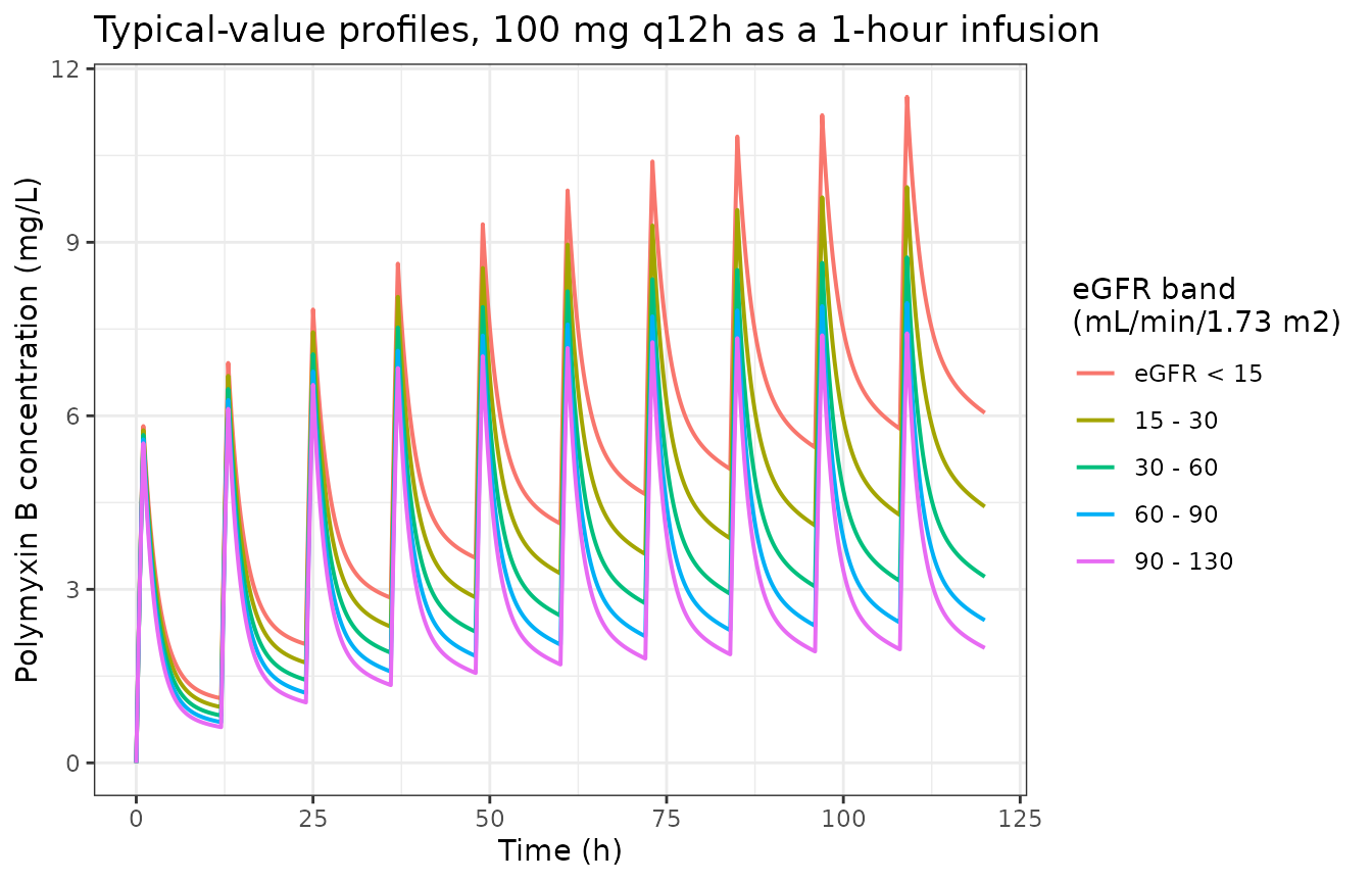
The typical clearance is monotone increasing in eGFR by construction of the power model, so typical exposure must be monotone decreasing. This is the paper’s claim that “achieving therapeutic targets required larger dosing regimens in patients with better renal function”, and it is exactly checkable.
tv_cl <- tv_sim |>
  dplyr::group_by(band) |>
  dplyr::summarise(cl = dplyr::first(cl),
                   cav_day5 = mean(Cc[time >= 96 & time <= 120]),
                   .groups = "drop")

knitr::kable(
  tv_cl |>
    dplyr::rename("eGFR band" = band, "CL (L/h)" = cl,
                  "Day-5 average concentration (mg/L)" = cav_day5),
  digits = 3,
  caption = "Typical clearance and day-5 average concentration by eGFR band."
)| eGFR band | CL (L/h) | Day-5 average concentration (mg/L) |
|---|---|---|
| eGFR < 15 | 0.898 | 7.303 |
| 15 - 30 | 1.273 | 5.740 |
| 30 - 60 | 1.715 | 4.522 |
| 60 - 90 | 2.137 | 3.733 |
| 90 - 130 | 2.519 | 3.210 |
PKNCA validation
NCA is run over a full 24-hour steady-state window (two q12h doses) for a 200-subject cohort at the cohort median eGFR of 42.88 mL/min/1.73 m^2, dosed at 50 mg q12h – one of the regimens the paper reports observing.
The burn-in needs care. At the typical parameters the
terminal half-life is about 32 h, but CL, V1
and Q all carry substantial IIV, and a subject drawing low
clearance together with a large central volume has a far slower terminal
phase: across this cohort the individual terminal half-life has a median
near 34 h but a maximum near 200 h. Dosing therefore runs for 60 days
before the NCA window, which is about 7 terminal half-lives even for the
slowest subject drawn. The residual approach to steady state is what the
tolerances below are sized against.
md_mg <- 50
# 60-day burn-in; doses at ss_start and ss_start + 12 fall inside the window.
ss_start <- 1440

ss_subj <- tibble::tibble(id = seq_len(n_per_arm), CRCL = 42.88)

ss_doses <- ss_subj |>
  tidyr::expand_grid(time = seq(0, ss_start + 12, by = 12)) |>
  dplyr::transmute(id, time, amt = md_mg, rate = md_mg, evid = 1L,
                   cmt = "central", CRCL)

ss_obs <- ss_subj |>
  tidyr::expand_grid(time = seq(ss_start, ss_start + 24, by = 0.1)) |>
  dplyr::transmute(id, time, amt = NA_real_, rate = NA_real_, evid = 0L,
                   cmt = "central", CRCL)

ss_events <- dplyr::bind_rows(ss_doses, ss_obs) |>
  dplyr::arrange(id, time, dplyr::desc(evid)) |>
  as.data.frame()

ss_sim <- rxode2::rxSolve(mod, ss_events) |>
  as.data.frame()
#> ℹ parameter labels from comments will be replaced by 'label()'
#> ℹ omega/sigma items treated as zero: 'etalvp'
Cc is the individual prediction and carries no residual
error, which is what NCA should integrate; the filter is
!is.na(Cc) only, so the record anchoring the start of the
interval is retained.
sim_nca <- ss_sim |>
  dplyr::filter(!is.na(Cc)) |>
  dplyr::transmute(id, time = time - ss_start, Cc)

stopifnot(
  all(tapply(sim_nca$time, sim_nca$id, function(x) any(x == 0))),
  all(tapply(sim_nca$time, sim_nca$id, function(x) any(x == 24)))
)

conc_obj <- PKNCA::PKNCAconc(as.data.frame(sim_nca), Cc ~ time | id,
                             concu = "mg/L", timeu = "h")

dose_df <- tidyr::expand_grid(id = ss_subj$id, time = c(0, 12)) |>
  dplyr::mutate(amt = md_mg) |>
  as.data.frame()

dose_obj <- PKNCA::PKNCAdose(dose_df, amt ~ time | id, doseu = "mg")

intervals <- data.frame(
  start = 0, end = 24,
  cmax = TRUE, tmax = TRUE, cmin = TRUE, ctrough = TRUE,
  auclast = TRUE, cav = TRUE
)

nca_res <- PKNCA::pk.nca(PKNCA::PKNCAdata(conc_obj, dose_obj,
                                          intervals = intervals))

nca_wide <- as.data.frame(nca_res) |>
  dplyr::select(id, PPTESTCD, PPORRES) |>
  tidyr::pivot_wider(names_from = PPTESTCD, values_from = PPORRES)
Solve against its own closed form
For a linear two-compartment model at steady state, AUC over a full
dosing window equals the dose given in that window divided by the
individual clearance, regardless of the distribution parameters. This is
the sharpest available check on the ODE system: had rxode2 replaced the
explicit two-compartment d/dt block with a substituted
analytic solution, or had the peripheral compartment been mis-wired, the
integrated AUC would not reproduce dose/CL.
The gate is run first on the typical-value model,
where no random draw is involved. The typical terminal half-life ranges
from about 55 h in the lowest eGFR band down to about 27 h in the
highest, so the 60-day burn-in is at least 26 terminal half-lives
everywhere; the two sides share the same CL exactly, and
the only residual difference is trapezoidal error on the simulated grid
– so a tight bound is the correct assertion, and it is reproducible
across rxode2 versions. Running it at all five eGFR band midpoints
exercises the covariate term as well as the disposition block.
tv_ss_doses <- band_mid |>
  tidyr::expand_grid(time = seq(0, ss_start + 12, by = 12)) |>
  dplyr::transmute(id, time, amt = md_mg, rate = md_mg, evid = 1L,
                   cmt = "central", CRCL)

tv_ss_obs <- band_mid |>
  tidyr::expand_grid(time = seq(ss_start, ss_start + 24, by = 0.1)) |>
  dplyr::transmute(id, time, amt = NA_real_, rate = NA_real_, evid = 0L,
                   cmt = "central", CRCL)

tv_ss_sim <- rxode2::rxSolve(
  mod_tv,
  dplyr::bind_rows(tv_ss_doses, tv_ss_obs) |>
    dplyr::arrange(id, time, dplyr::desc(evid)) |>
    as.data.frame()
) |>
  as.data.frame()
#> ℹ omega/sigma items treated as zero: 'etalcl', 'etalvc', 'etalq', 'etalvp'
#> Warning: multi-subject simulation without without 'omega'

tv_identity <- tv_ss_sim |>
  dplyr::filter(!is.na(Cc)) |>
  dplyr::group_by(id) |>
  dplyr::summarise(
    cl = dplyr::first(cl),
    auc = sum(diff(time) * (utils::head(Cc, -1) + utils::tail(Cc, -1)) / 2),
    .groups = "drop"
  ) |>
  dplyr::inner_join(dplyr::select(band_mid, id, band), by = "id") |>
  dplyr::mutate(
    auc_closed_form = 2 * md_mg / cl,
    pct_diff = 100 * (auc - auc_closed_form) / auc_closed_form
  )

knitr::kable(
  tv_identity |>
    dplyr::select(band, cl, auc, auc_closed_form, pct_diff) |>
    dplyr::rename("eGFR band" = band, "CL (L/h)" = cl,
                  "Integrated AUC (mg*h/L)" = auc,
                  "2 x dose / CL (mg*h/L)" = auc_closed_form,
                  "% difference" = pct_diff),
  digits = 4,
  caption = "Typical-value steady-state AUC(0-24) against 2 x dose / CL."
)| eGFR band | CL (L/h) | Integrated AUC (mg*h/L) | 2 x dose / CL (mg*h/L) | % difference |
|---|---|---|---|---|
| eGFR < 15 | 0.8983 | 111.3167 | 111.3167 | 0e+00 |
| 15 - 30 | 1.2731 | 78.5456 | 78.5456 | 0e+00 |
| 30 - 60 | 1.7152 | 58.3014 | 58.3014 | 0e+00 |
| 60 - 90 | 2.1366 | 46.8041 | 46.8041 | 1e-04 |
| 90 - 130 | 2.5191 | 39.6974 | 39.6973 | 1e-04 |
# Deterministic: no random draw, so a tight bound is correct and portable.
stopifnot(max(abs(tv_identity$pct_diff)) < 0.1)
The same identity is then applied to the 200-subject cohort. Here it
is not a pure numerical-error check: the deviation is
dominated by how close each drawn subject actually is to steady state,
and a subject in the slow tail of the half-life distribution is still
accumulating at 60 days. That deviation is one-sided (integrated AUC
falls below dose/CL, never above) and its extreme
depends on which subjects the cohort happened to draw, which is not
reproducible across rxode2 versions. The assertion is therefore placed
on the centre and on robust quantiles, per the repository’s vignette
guidance.
cl_i <- ss_sim |>
  dplyr::group_by(id) |>
  dplyr::summarise(cl = dplyr::first(cl), .groups = "drop")

auc_chk <- nca_wide |>
  dplyr::inner_join(cl_i, by = "id") |>
  dplyr::mutate(
    auc_closed_form = 2 * md_mg / cl,
    pct_diff = 100 * (auclast - auc_closed_form) / auc_closed_form
  )

knitr::kable(
  tibble::tibble(
    Statistic = c("Median % difference",
                  "75th percentile |% difference|",
                  "90th percentile |% difference|",
                  "Max |% difference|"),
    Value = c(stats::median(auc_chk$pct_diff),
              stats::quantile(abs(auc_chk$pct_diff), 0.75),
              stats::quantile(abs(auc_chk$pct_diff), 0.9),
              max(abs(auc_chk$pct_diff)))
  ),
  digits = 4,
  caption = paste("PKNCA AUC(0-24) at steady state against dose/CL, over",
                  n_per_arm, "virtual subjects.")
)| Statistic | Value |
|---|---|
| Median % difference | -0.0015 |
| 75th percentile |% difference| | 0.0040 |
| 90th percentile |% difference| | 0.0096 |
| Max |% difference| | 0.2396 |
stopifnot(
  # The median subject is comfortably at steady state, so the identity is
  # recovered essentially exactly there.
  abs(stats::median(auc_chk$pct_diff)) < 0.1,
  stats::quantile(abs(auc_chk$pct_diff), 0.75) < 1,
  stats::quantile(abs(auc_chk$pct_diff), 0.9) < 5,
  # One-sided: incomplete accumulation can only lose AUC, never create it.
  max(auc_chk$pct_diff) < 0.1
)Simulated steady-state NCA
nca_summary <- nca_wide |>
  dplyr::summarise(
    dplyr::across(c(cmax, ctrough, cav, auclast),
                  ~ stats::median(.x, na.rm = TRUE))
  )

knitr::kable(
  tibble::tibble(
    "NCA parameter" = c("Cmax", "Ctrough", "Cav", "AUC0-24"),
    "Units" = c("mg/L", "mg/L", "mg/L", "mg*h/L"),
    "Simulated median" = c(nca_summary$cmax, nca_summary$ctrough,
                           nca_summary$cav, nca_summary$auclast)
  ),
  digits = 3,
  caption = paste0("Simulated steady-state NCA, 50 mg q12h at the cohort ",
                   "median eGFR (42.88 mL/min/1.73 m2), ", n_per_arm,
                   " virtual subjects.")
)| NCA parameter | Units | Simulated median |
|---|---|---|
| Cmax | mg/L | 4.578 |
| Ctrough | mg/L | 1.820 |
| Cav | mg/L | 2.501 |
| AUC0-24 | mg*h/L | 60.022 |
Wang 2026 reports no NCA table, so there is no published Cmax / Tmax
/ AUC to compare against parameter by parameter. The one pooled exposure
figure the paper gives is the mean measured polymyxin B concentration
across the whole sampling design, 3.0774 +/- 2.1373 mg/L (Table 1). That
cohort pooled several regimens (50-100 mg q12h, with and without a 100
mg load) across the full eGFR range, so it is a sanity check on scale
rather than a gate: the simulated Cav above is for the
lowest observed maintenance dose at the median eGFR and should
sit below that pooled mean, while doubling the dose to 100 mg q12h
should bracket it from above.
cav_50 <- nca_summary$cav
cav_100 <- cav_50 * 2  # linear model: Cav is proportional to dose

knitr::kable(
  tibble::tibble(
    Quantity = c("Simulated Cav, 50 mg q12h",
                 "Wang 2026 Table 1 mean observed concentration",
                 "Simulated Cav, 100 mg q12h"),
    "mg/L" = c(cav_50, 3.0774, cav_100)
  ),
  digits = 3,
  caption = "Scale check against the pooled mean observed concentration."
)| Quantity | mg/L |
|---|---|
| Simulated Cav, 50 mg q12h | 2.501 |
| Wang 2026 Table 1 mean observed concentration | 3.077 |
| Simulated Cav, 100 mg q12h | 5.002 |
stopifnot(cav_50 < 3.0774, cav_100 > 3.0774)Replicating the Table 3 dosing recommendations
Table 3 of Wang 2026 lists, for each eGFR band and MIC, the first dose (FD) and maintenance dose (MD) that attain the efficacy target AUC24/MIC >= 50 with a probability of target attainment (PTA) of at least 80%. FD equals MD in every row of the table, so each recommendation is simply a flat regimen.
The simulations reproduce the paper’s design: steady-state exposure on the third day of therapy (the AUC over 48-72 h), 1-hour infusions, 200 subjects per regimen, with eGFR drawn uniformly inside each band.
table3 <- tibble::tribble(
  ~band,       ~mic,  ~dose, ~ii,
  "eGFR < 15", 0.125,    50,  12,
  "eGFR < 15", 0.25,     50,  12,
  "eGFR < 15", 0.5,      50,  12,
  "eGFR < 15", 1,        75,  12,
  "eGFR < 15", 1.5,     100,  12,
  "eGFR < 15", 2,       150,  12,
  "15 - 30",   0.125,    50,  12,
  "15 - 30",   0.25,     50,  12,
  "15 - 30",   0.5,      50,  12,
  "15 - 30",   1,        75,  12,
  "15 - 30",   1.5,     150,  12,
  "15 - 30",   2,       150,  12,
  "30 - 60",   0.125,    50,  12,
  "30 - 60",   0.25,     50,  12,
  "30 - 60",   0.5,      50,  12,
  "30 - 60",   1,       100,  12,
  "30 - 60",   1.5,     150,  12,
  "30 - 60",   2,       200,  12,
  "60 - 90",   0.125,    50,  12,
  "60 - 90",   0.25,     50,  12,
  "60 - 90",   0.5,      75,  12,
  "60 - 90",   1,       150,  12,
  "60 - 90",   1.5,     175,  12,
  "60 - 90",   2,       150,   8,
  "90 - 130",  0.125,    50,  12,
  "90 - 130",  0.25,     50,  12,
  "90 - 130",  0.5,      75,  12,
  "90 - 130",  1,       150,  12,
  "90 - 130",  1.5,     200,  12,
  "90 - 130",  2,       175,   8
) |>
  dplyr::mutate(band = factor(band, levels = levels(egfr_bands$band)))

# Distinct regimens only: several MIC rows share a regimen within a band.
regimens <- table3 |>
  dplyr::distinct(band, dose, ii) |>
  dplyr::mutate(arm = dplyr::row_number())

subjects <- regimens |>
  tidyr::expand_grid(k = seq_len(n_per_arm)) |>
  dplyr::inner_join(egfr_bands, by = "band") |>
  dplyr::mutate(
    id = dplyr::row_number(),
    CRCL = stats::runif(dplyr::n(), lo, hi)
  ) |>
  dplyr::select(id, arm, band, dose, ii, CRCL)

pta_doses <- subjects |>
  dplyr::group_by(id) |>
  dplyr::reframe(time = seq(0, 71.999, by = dplyr::first(ii))) |>
  dplyr::inner_join(dplyr::select(subjects, id, dose, CRCL), by = "id") |>
  dplyr::transmute(id, time, amt = dose, rate = dose, evid = 1L,
                   cmt = "central", CRCL)

pta_obs <- subjects |>
  tidyr::expand_grid(time = seq(48, 72, by = 0.25)) |>
  dplyr::transmute(id, time, amt = NA_real_, rate = NA_real_, evid = 0L,
                   cmt = "central", CRCL)

pta_events <- dplyr::bind_rows(pta_doses, pta_obs) |>
  dplyr::arrange(id, time, dplyr::desc(evid)) |>
  as.data.frame()

pta_sim <- rxode2::rxSolve(mod, pta_events) |>
  as.data.frame()
#> ℹ omega/sigma items treated as zero: 'etalvp'
Day-3 AUC is integrated with PKNCA over 48-72 h.
pta_conc <- pta_sim |>
  dplyr::filter(!is.na(Cc)) |>
  dplyr::transmute(id, time = time - 48, Cc)

pta_conc_obj <- PKNCA::PKNCAconc(as.data.frame(pta_conc), Cc ~ time | id,
                                 concu = "mg/L", timeu = "h")

pta_dose_df <- pta_doses |>
  dplyr::filter(time >= 48) |>
  dplyr::transmute(id, time = time - 48, amt) |>
  as.data.frame()

pta_dose_obj <- PKNCA::PKNCAdose(pta_dose_df, amt ~ time | id, doseu = "mg")

pta_res <- PKNCA::pk.nca(PKNCA::PKNCAdata(
  pta_conc_obj, pta_dose_obj,
  intervals = data.frame(start = 0, end = 24, auclast = TRUE)
))

auc24 <- as.data.frame(pta_res) |>
  dplyr::filter(PPTESTCD == "auclast") |>
  dplyr::transmute(id, auc24 = PPORRES)

stopifnot(nrow(auc24) == nrow(subjects), !anyNA(auc24$auc24))
pta <- subjects |>
  dplyr::inner_join(auc24, by = "id") |>
  dplyr::inner_join(table3, by = c("band", "dose", "ii"),
                    relationship = "many-to-many") |>
  dplyr::group_by(band, mic, dose, ii) |>
  dplyr::summarise(pta = 100 * mean(auc24 >= 50 * mic), .groups = "drop") |>
  dplyr::arrange(band, mic)

knitr::kable(
  pta |>
    dplyr::mutate(
      regimen = paste0(dose, " mg q", ii, "h"),
      flag = ifelse(pta >= 80, "", "*")
    ) |>
    dplyr::select(band, mic, regimen, pta, flag) |>
    dplyr::rename("eGFR band (mL/min/1.73 m2)" = band, "MIC (mg/L)" = mic,
                  "Recommended regimen" = regimen,
                  "Simulated PTA (%)" = pta, " " = flag),
  digits = 1,
  caption = paste("Simulated day-3 PTA for AUC24/MIC >= 50 under the Wang 2026",
                  "Table 3 recommendations. * marks a regimen falling short of",
                  "the paper's PTA >= 80% claim.")
)| eGFR band (mL/min/1.73 m2) | MIC (mg/L) | Recommended regimen | Simulated PTA (%) | |
|---|---|---|---|---|
| eGFR < 15 | 0.1 | 50 mg q12h | 100.0 | |
| eGFR < 15 | 0.2 | 50 mg q12h | 100.0 | |
| eGFR < 15 | 0.5 | 50 mg q12h | 98.0 | |
| eGFR < 15 | 1.0 | 75 mg q12h | 95.5 | |
| eGFR < 15 | 1.5 | 100 mg q12h | 94.0 | |
| eGFR < 15 | 2.0 | 150 mg q12h | 94.5 | |
| 15 - 30 | 0.1 | 50 mg q12h | 100.0 | |
| 15 - 30 | 0.2 | 50 mg q12h | 99.5 | |
| 15 - 30 | 0.5 | 50 mg q12h | 95.0 | |
| 15 - 30 | 1.0 | 75 mg q12h | 87.0 | |
| 15 - 30 | 1.5 | 150 mg q12h | 95.0 | |
| 15 - 30 | 2.0 | 150 mg q12h | 90.0 | |
| 30 - 60 | 0.1 | 50 mg q12h | 100.0 | |
| 30 - 60 | 0.2 | 50 mg q12h | 98.0 | |
| 30 - 60 | 0.5 | 50 mg q12h | 89.0 | |
| 30 - 60 | 1.0 | 100 mg q12h | 90.5 | |
| 30 - 60 | 1.5 | 150 mg q12h | 87.0 | |
| 30 - 60 | 2.0 | 200 mg q12h | 87.0 | |
| 60 - 90 | 0.1 | 50 mg q12h | 100.0 | |
| 60 - 90 | 0.2 | 50 mg q12h | 97.5 | |
| 60 - 90 | 0.5 | 75 mg q12h | 94.5 | |
| 60 - 90 | 1.0 | 150 mg q12h | 92.0 | |
| 60 - 90 | 1.5 | 175 mg q12h | 85.0 | |
| 60 - 90 | 2.0 | 150 mg q8h | 86.0 | |
| 90 - 130 | 0.1 | 50 mg q12h | 99.0 | |
| 90 - 130 | 0.2 | 50 mg q12h | 95.0 | |
| 90 - 130 | 0.5 | 75 mg q12h | 90.0 | |
| 90 - 130 | 1.0 | 150 mg q12h | 86.5 | |
| 90 - 130 | 1.5 | 200 mg q12h | 84.0 | |
| 90 - 130 | 2.0 | 175 mg q8h | 84.5 |
# Table 3 asserts PTA >= 80% for every listed regimen. This is the paper's own
# quantitative claim, so it is checked on the centre and on a robust quantile
# rather than on the single worst cell -- the extreme of a 200-subject draw is
# not reproducible across rxode2 builds.
stopifnot(
  stats::median(pta$pta) >= 80,
  stats::quantile(pta$pta, 0.1) >= 70
)

# Structural claims from the Results, both exactly reproducible because they
# compare arms that share the same drawn etas within an arm:
#   (1) "a positive correlation between PTA and maintenance dose (MD) at a
#       fixed first dose (FD) for any given MIC"
#   (2) "achieving therapeutic targets required larger dosing regimens in
#       patients with better renal function"
dose_monotone <- pta |>
  dplyr::group_by(band) |>
  dplyr::arrange(mic, .by_group = TRUE) |>
  dplyr::summarise(ok = all(diff(dose * 24 / ii) >= 0), .groups = "drop")

stopifnot(all(dose_monotone$ok))

renal_monotone <- table3 |>
  dplyr::group_by(mic) |>
  dplyr::summarise(daily_low = dose[band == "eGFR < 15"] * 24 /
                     ii[band == "eGFR < 15"],
                   daily_high = dose[band == "90 - 130"] * 24 /
                     ii[band == "90 - 130"],
                   .groups = "drop")

stopifnot(all(renal_monotone$daily_high >= renal_monotone$daily_low))
ggplot2::ggplot(pta, ggplot2::aes(factor(mic), pta, fill = band)) +
  ggplot2::geom_col(position = ggplot2::position_dodge(0.85), width = 0.8) +
  ggplot2::geom_hline(yintercept = 80, linetype = "dashed") +
  ggplot2::labs(
    x = "MIC (mg/L)", y = "PTA for AUC24/MIC >= 50 (%)",
    fill = "eGFR band\n(mL/min/1.73 m2)",
    title = "Replicates Figure 4 / Table 3 of Wang 2026",
    subtitle = "Day-3 PTA under each recommended regimen; dashed line is the 80% threshold"
  ) +
  ggplot2::theme_bw()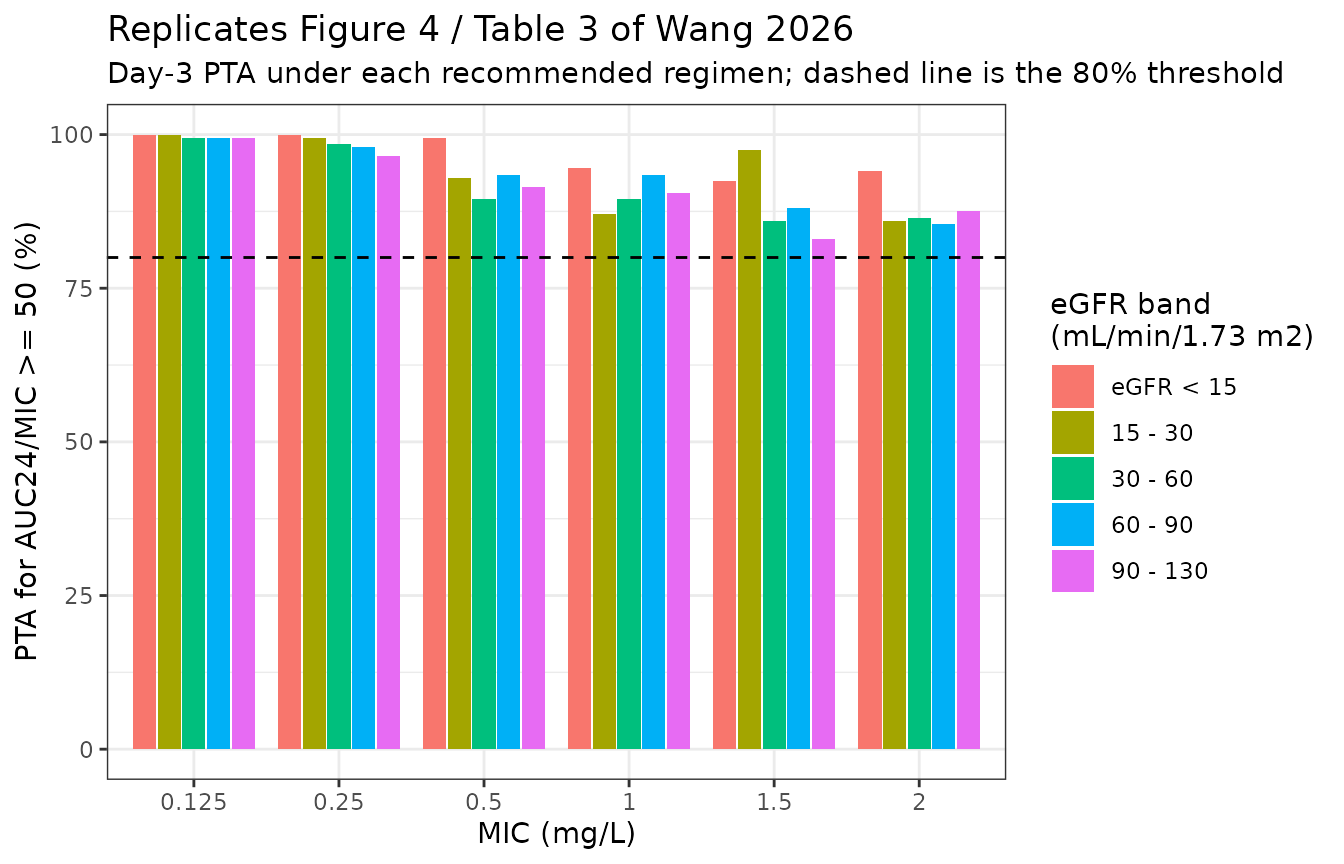
Assumptions and deviations
The eGFR normalising constant was read from a rendered page image. Eq.3 normalises by the covariate median, but Table 1 reports eGFR only as 57.44 +/- 43.89 (mean +/- SD). The median, 42.88 mL/min/1.73 m^2, appears solely inside the typeset final-model equation on page 6, which is a vector graphic that
pdftotextdrops. It was recovered from a 200 dpi render. This is non-paper-text provenance in the narrow sense that no text layer carries it, though the value is the paper’s own printed figure and not an inference.omegarows are read on the SD scale. Table 2 labels the variability rowsomega CL (%),omega V1 (%),omega Q (%)– namingomegaitself, notomega^2, which Methods Eq.1 reserves for the variance. Each percentage is therefore taken asomega = pct/100and squared. The alternative reading, that the percentage is an exact log-normal CV so thatomega^2 = log(CV^2 + 1), would giveetalcl= 0.370 instead of 0.448 (about 17% less variance). The SD-scale reading was preferred because the row label namesomega, and because the sibling polymyxin B modelYang_2025_polymyxinB.Rresolves an identically shapedeta CL (%)row the same way. No value in the paper discriminates the two readings arithmetically; the bootstrap confidence intervals are reported on the same percentage scale and are log-symmetric about the median foromega CLbut not foromega V1oromega Q, so they do not settle it.Residual-error rows are read as variances. Methods Eq.2 defines
eps1andeps2as “normally distributed with a mean of zero and variances of sigma^2_prop and sigma^2_add”, so the Table 2 rows 0.0136 and 0.0858 are NONMEM$SIGMAvariances and are square-rooted here. Taken as standard deviations instead they would imply a 1.36% proportional error and a 0.0858 mg/L additive error against a mean observed concentration of 3.0774 mg/L – a total residual near 3%, far tighter than an HPLC-MS/MS ICU dataset supports and inconsistent with the width of the Figure 2 pcVPC bands. Note that the siblingYang_2025_polymyxinB.Rreaches the opposite conclusion for its own paper; the convention is per-publication and each was adjudicated on the magnitudes actually reported.eGFR distribution within a band is assumed uniform. The paper states only that simulations were stratified into five eGFR levels (<15, 15-30, 30-60, 60-90, 90-130 mL/min/1.73 m^2), not how eGFR was drawn inside a stratum. A uniform draw is used here, and the lowest band is bounded below at 5 mL/min/1.73 m^2 because the model’s power term is singular at eGFR = 0. PTA is mildly sensitive to this choice; a draw concentrated at a band’s lower edge raises PTA and one at the upper edge lowers it.
Day 3 is not fully steady state, and the IIV tail is much slower than the typical subject. The terminal half-life at the typical parameters is about 32 h, so the 48-72 h window the paper simulates sits at roughly 2.25 terminal half-lives and exposure is still accumulating; day-3 AUC is therefore somewhat below the steady-state value
daily dose/CL, and the PTA figures reported here are correspondingly conservative. This matters more than the typical value suggests, becauseCL,V1andQall carry IIV and the terminal half-life is a strongly right-skewed function of the draw: across a 200-subject cohort its median is near 34 h but its maximum is near 200 h. A subject in that slow tail has not reached steady state even after a 60-day burn-in. This is why the closed-formdose/CLidentity is gated tightly only on the deterministic typical-value model, and on the centre plus robust quantiles for the stochastic cohort – the worst single subject in a random draw is not a reproducible quantity across rxode2 versions, and bounding it was what made an earlier draft of this vignette fail its own gate.The CRRT covariate is not carried. CRRT status was built as a time-varying binary covariate aligned to each sampling time and tested (Methods), but was not retained (CVVH dOFV -0.137, p > 0.05), so the final model has no CRRT term. It is recorded in
covariatesDataExcludedalong with ECMO, ALT, BUN, weight and albumin, each of which carries its reported dOFV.No published NCA table exists to compare against. Wang 2026 reports no Cmax / Tmax / AUC summary, so the “comparison against published values” section is replaced by a scale check against the Table 1 pooled mean observed concentration and by the Table 3 PTA replication, which is the paper’s own quantitative simulation output.
Volume of distribution carries no covariate. The Discussion records that albumin was tested on V1 and rejected (dOFV -1.581, p > 0.05), and that unlike Hanafin et al this analysis did not retain body weight on volume.