Model and source
- Citation: Li A, Mak WY, Ruan T, Dong F, Zheng N, Gu M, Guo W, Zhang J, Cheng H, Ruan C, Shi Y, Zang Y, Zhu X, He Q, Xiang X, Wang G, Zhu X. Population pharmacokinetics of Amisulpride in Chinese patients with schizophrenia with external validation: the impact of renal function. Front Pharmacol. 2023;14:1215065. doi:10.3389/fphar.2023.1215065.
- Description: Population PK model for oral amisulpride in Chinese adults with schizophrenia (Li 2023). One-compartment disposition with first-order absorption and linear elimination, parameterised on the apparent (oral) scale as CL/F and V/F. Renal function, as the race-free CKD-EPI estimated glomerular filtration rate (mL/min/1.73 m^2), was included a priori in the structural model and enters CL/F as a power function centred on 113.84 mL/min/1.73 m^2; no other covariate was retained. Exponential inter-individual variability on CL/F and V/F (none on Ka) and a combined additive plus proportional residual error. Developed on 776 therapeutic-drug-monitoring patients and externally validated on a further 145.
- Article: https://doi.org/10.3389/fphar.2023.1215065 (open access)
Li 2023 developed a one-compartment population PK model for oral amisulpride from routine therapeutic-drug-monitoring (TDM) samples in Chinese adults with schizophrenia, with renal function built into the structural model a priori, and externally validated it on a separate cohort. The model is then used to simulate six common twice-daily regimens at three levels of renal function (Figure 6) and the effect of eGFR on steady-state exposure (Figure 4). Both analyses are reproduced below.
Population
The model was fitted to the development cohort of 776 patients (on average 3 random TDM samples each) treated at Beijing Anding Hospital between December 2018 and March 2022; a further 145 patients admitted before 15 November 2019 formed the external validation cohort (Li 2023 Table 1). In the development cohort the median age was 33 years (IQR 23-47), median weight 66 kg (IQR 57-79), 61.2% were female and 96.4% were Han Chinese. Renal function was mostly normal or supranormal: CKD-EPI eGFR (no race component) median 114 (IQR 101-130) mL/min/1.73 m^2, 89.0% CKD stage G1, 25.4% above 130 mL/min/1.73 m^2 and only five patients in stage G3a. Daily doses averaged 566 +/- 264 mg (median 575); 12.4% of patients also received lithium.
pop <- rxode2::rxode(readModelDb("Li_2023_amisulpride"))$population
#> ℹ parameter labels from comments will be replaced by 'label()'
str(pop[c("n_subjects", "age_range", "weight_range", "dose_range", "renal_function")])
#> List of 5
#>  $ n_subjects    : int 776
#>  $ age_range     : chr "Median 33 years (IQR 23-47) in the development cohort (Li 2023 Table 1)"
#>  $ weight_range  : chr "Median 66 kg (IQR 57-79) in the development cohort (Li 2023 Table 1)"
#>  $ dose_range    : chr "Oral amisulpride, daily dose 50-1220 mg across both cohorts (development cohort mean 566 +/- 264, median 575 mg"| __truncated__
#>  $ renal_function: chr "CKD-EPI eGFR (no race component) median 114 (IQR 101-130) mL/min/1.73 m^2 in the development cohort; 25.4 perce"| __truncated__
Source trace
Every ini() value carries an in-file comment in
inst/modeldb/specificDrugs/Li_2023_amisulpride.R; the table
collects them.
| Equation / parameter | Value | Source location |
|---|---|---|
| Structure: 1 compartment, first-order absorption, linear elimination | n/a | Results 3.2; Supplementary Table S2 (model 9 ‘Ami final’);
Supplementary Figure S6 (ADVAN2 TRANS2) |
lka (Ka) |
0.106 1/h | Table 2, RSE 12%; bootstrap 0.106 [0.0916-0.1210] |
lcl (CL/F) |
60.5 L/h | Table 2, RSE 2%; bootstrap 60.4 [58.62-62.37] |
lvc (V/F) |
645 L | Table 2, RSE 18%; bootstrap 650 [521.3-769.6] |
e_crcl_cl (eGFR exponent on CL/F) |
0.817 | Table 2 row ‘eGFR on CL/F RCL’, RSE 10%; bootstrap 0.821 [0.7030-0.9319] |
CL/F = 60.5 * (eGFR/113.84)^0.817 |
centring 113.84 | Table 2 footnote equation; Supplementary Figure S6
TVCL = THETA(1)*(GFR_CKD/113.84)**THETA(6)
|
| eGFR definition | CKD-EPI, race-free | Table 1 footnote; Supplementary Table S1 |
etalcl |
log(1 + 0.359^2) |
Table 2, IIV CL/F 35.9% CV (RSE 7%, shrinkage 20%); exponential form from Methods Eq. 1 and Supplementary Figure S6 |
etalvc |
log(1 + 1.309^2) |
Table 2, IIV V/F 130.9% CV (RSE 25%, shrinkage 46%) |
| No IIV on Ka | n/a | Supplementary Figure S6 $OMEGA ... 0 FIX; IIV KA
|
propSd |
0.346 | Table 2 ‘Prop.RE’ 34.6% (RSE 3%) |
addSd |
13.7 ng/mL | Table 2 ‘Add.RE’ 13.7 (RSE 36%) |
| Combined error on the variance scale | n/a | Supplementary Figure S6
W = SQRT(THETA(4)**2*IPRED**2 + THETA(5)**2)
|
Cc = central / vc * 1000 |
n/a | Supplementary Figure S6 S2 = V/1000 (dose in mg,
concentration in ng/mL) |
The IIV scale
Table 2 prints the between-subject variability only as a percent CV,
and the paper does not say how the CV was computed. For an exponential
eta the two usual conventions are
CV = sqrt(exp(omega^2) - 1) and
CV = sqrt(omega^2). They nearly agree for CL/F but not for
the large V/F variability:
tibble::tibble(
  parameter = c("CL/F", "V/F"),
  cv_pct = c(35.9, 130.9)
) |>
  mutate(
    omega2_exact = log(1 + (cv_pct / 100)^2),
    omega2_sqrt = (cv_pct / 100)^2
  ) |>
  dplyr::rename(
    "Parameter" = parameter,
    "Published CV (%)" = cv_pct,
    "omega^2 = log(1 + CV^2) (packaged)" = omega2_exact,
    "omega^2 = CV^2 (alternative)" = omega2_sqrt
  ) |>
knitr::kable(digits = 4)| Parameter | Published CV (%) | omega^2 = log(1 + CV^2) (packaged) | omega^2 = CV^2 (alternative) |
|---|---|---|---|
| CL/F | 35.9 | 0.1212 | 0.1289 |
| V/F | 130.9 | 0.9982 | 1.7135 |
The control stream in Supplementary Figure S6 does not settle it: its
$OMEGA starting values (0.187 and 0.5) are round numbers
far from either reading, as are its $THETA starting values
(60, 700, 0.1, 0.35, 18). The maintainers therefore used
log(1 + CV^2), the convention used across this package. The
choice matters only for the spread of V/F, which in a model with slow
absorption (Ka 0.106 1/h) affects mainly the within-interval
fluctuation; the TDM cohort check below
shows that the observed dose-normalised concentration distribution
cannot tell the two readings apart.
Figure 6: six regimens at three levels of renal function
Li 2023 simulated each regimen for 8 days (morning dose at 0 h every 24 h, evening dose at 12 h every 24 h) and plotted the last 24 h (144-168 h) at eGFR 50, 100 and 200 mL/min/1.73 m^2 (Supplementary Figure S7). The simulation below follows that design with 100 virtual subjects per regimen and eGFR level, sampling IIV on CL/F and V/F.
regimens <- tibble::tibble(
  regimen = c(
    "100 mg + 100 mg", "100 mg + 200 mg", "200 mg + 200 mg",
    "200 mg + 400 mg", "400 mg + 400 mg", "600 mg + 600 mg"
  ),
  dose_am = c(100, 100, 200, 200, 400, 600),
  dose_pm = c(100, 200, 200, 400, 400, 600)
) |>
  mutate(regimen = factor(regimen, levels = regimen))

# Explicit dose rows (no addl) so the same table feeds rxSolve and PKNCA.
make_events <- function(subj, obs_times, last_dose = 156) {
  am <- subj |>
    tidyr::expand_grid(time = seq(0, last_dose, by = 24)) |>
    mutate(amt = dose_am)
  pm <- subj |>
    tidyr::expand_grid(time = seq(12, last_dose, by = 24)) |>
    mutate(amt = dose_pm)
  doses <- bind_rows(am, pm) |>
    mutate(evid = 1L, cmt = "depot")
  obs <- subj |>
    tidyr::expand_grid(time = obs_times) |>
    mutate(amt = NA_real_, evid = 0L, cmt = "central")
  bind_rows(doses, obs) |>
    arrange(id, time, desc(evid)) |>
    select(id, time, amt, evid, cmt, CRCL, regimen, egfr_label)
}

egfr_levels <- c(50, 100, 200)
egfr_names <- c(
  "eGFR 50 (mild-to-moderate impairment)",
  "eGFR 100 (normal)",
  "eGFR 200 (hyperfiltration)"
)
n_per_cell <- 100L

subj_fig6 <- tidyr::expand_grid(
  regimens,
  CRCL = egfr_levels,
  rep = seq_len(n_per_cell)
) |>
  mutate(
    id = dplyr::row_number(),
    egfr_label = factor(egfr_names[match(CRCL, egfr_levels)], levels = egfr_names)
  )

obs_ss <- seq(144, 168, by = 0.5)
ev_fig6 <- make_events(subj_fig6, obs_ss)
mod <- readModelDb("Li_2023_amisulpride")
rxode2::rxSetSeed(20230915)
sim_fig6 <- rxode2::rxSolve(
  mod,
  events = ev_fig6,
  keep = c("regimen", "egfr_label")
) |>
  as.data.frame()
#> ℹ parameter labels from comments will be replaced by 'label()'
band_df <- tibble::tibble(
  ymin = c(50, 100, 320, 640),
  ymax = c(100, 320, 640, 5000),
  zone = c("below range", "AGNP range", "above range", "above alert level")
)

# `sim` is the simulated observation (IIV plus residual error).
fig6_q <- sim_fig6 |>
  filter(!is.na(Cc)) |>
  group_by(egfr_label, regimen, time) |>
  summarise(
    Q05 = quantile(sim, 0.05),
    Q50 = median(sim),
    Q95 = quantile(sim, 0.95),
    ipred_Q05 = quantile(Cc, 0.05),
    ipred_Q50 = median(Cc),
    ipred_Q95 = quantile(Cc, 0.95),
    .groups = "drop"
  )

fig6_q |>
  mutate(tss = time - 144) |>
  ggplot(aes(tss, Q50)) +
  geom_rect(
    data = band_df,
    aes(xmin = -Inf, xmax = Inf, ymin = ymin, ymax = ymax, fill = zone),
    inherit.aes = FALSE, alpha = 0.15
  ) +
  geom_line(aes(colour = egfr_label)) +
  geom_line(aes(y = Q05, colour = egfr_label), linetype = "dotted") +
  geom_line(aes(y = Q95, colour = egfr_label), linetype = "dotted") +
  facet_grid(regimen ~ egfr_label) +
  scale_y_log10(breaks = c(50, 100, 320, 640, 1000, 2000, 5000)) +
  scale_x_continuous(breaks = c(0, 6, 12, 18, 24)) +
  scale_fill_manual(values = c(
    "below range" = "grey60", "AGNP range" = "green3",
    "above range" = "gold", "above alert level" = "red"
  )) +
  labs(
    x = "Time at steady state (h)", y = "Amisulpride (ng/mL)",
    colour = NULL, fill = NULL,
    caption = "Replicates Figure 6 of Li 2023: median (solid) and 5th-95th percentiles (dotted)."
  ) +
  theme_bw(base_size = 9) +
  theme(legend.position = "bottom", legend.box = "vertical")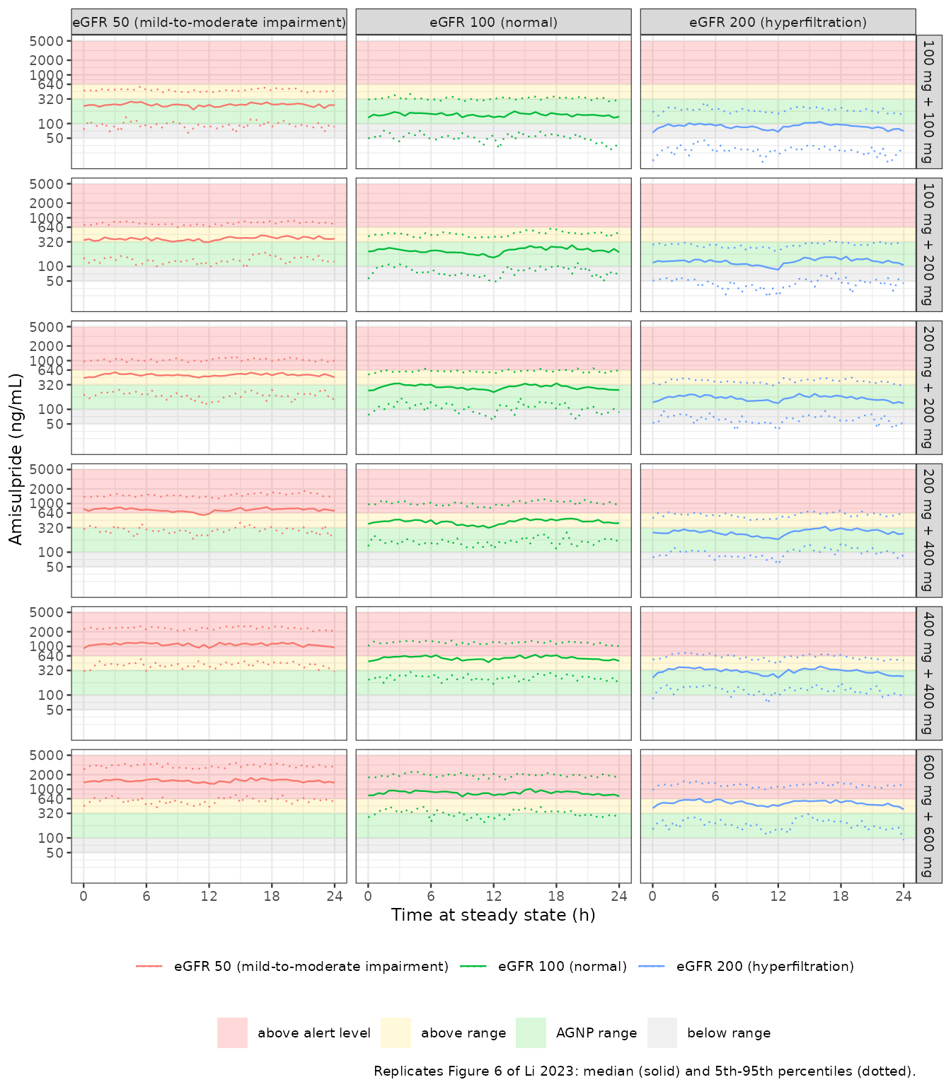
The pattern matches Figure 6: the median sits in the AGNP range (100-320 ng/mL) for 200 mg/day at eGFR 50 and 100 and below it at eGFR 200; it crosses the 640 ng/mL alert level at 800 mg/day only with impaired renal function.
The paper does not say whether its Figure 6 bands include residual error. Read by eye off Figure 6B (eGFR 100), the 95th percentile is about 2.3 times the median and the 5th percentile about 0.5 times. The upper band is reproduced only when residual error is included, so the plot above includes it; the lower band falls between the two versions:
fig6_q |>
  group_by(egfr_label) |>
  summarise(
    up_obs = mean(Q95 / Q50),
    lo_obs = mean(Q05 / Q50),
    up_ipred = mean(ipred_Q95 / ipred_Q50),
    lo_ipred = mean(ipred_Q05 / ipred_Q50)
  ) |>
  dplyr::rename(
    "Renal function" = egfr_label,
    "Q95/median, with residual" = up_obs,
    "Q05/median, with residual" = lo_obs,
    "Q95/median, IIV only" = up_ipred,
    "Q05/median, IIV only" = lo_ipred
  ) |>
knitr::kable(digits = 2, caption = "Band width relative to the median, averaged over regimens and times.")| Renal function | Q95/median, with residual | Q05/median, with residual | Q95/median, IIV only | Q05/median, IIV only |
|---|---|---|---|---|
| eGFR 50 (mild-to-moderate impairment) | 2.06 | 0.38 | 1.69 | 0.58 |
| eGFR 100 (normal) | 2.21 | 0.38 | 1.79 | 0.57 |
| eGFR 200 (hyperfiltration) | 2.19 | 0.37 | 1.90 | 0.57 |
PKNCA validation
PKNCA is run on the steady-state dosing interval (144-168 h) of the
typical patient (random effects set to zero) for every regimen and eGFR
level. Because both sides use the same parameters, the average
concentration must equal the closed form
Cav = daily dose / (24 * CL/F) up to trapezoidal error, and
the assertion is tight.
subj_typ <- tidyr::expand_grid(regimens, CRCL = egfr_levels) |>
  mutate(
    id = dplyr::row_number(),
    egfr_label = factor(egfr_names[match(CRCL, egfr_levels)], levels = egfr_names)
  )
ev_typ <- make_events(subj_typ, obs_ss)

sim_typ <- rxode2::rxSolve(
  rxode2::zeroRe(mod),
  events = ev_typ,
  keep = c("regimen", "egfr_label")
) |>
  as.data.frame()
#> ℹ parameter labels from comments will be replaced by 'label()'
#> ℹ omega/sigma items treated as zero: 'etalcl', 'etalvc'
#> Warning: multi-subject simulation without without 'omega'
conc_ss <- sim_typ |>
  filter(!is.na(Cc)) |>
  select(id, time, Cc, regimen, egfr_label)

dose_ss <- ev_typ |>
  filter(evid == 1) |>
  select(id, time, amt, regimen, egfr_label)

conc_obj <- PKNCA::PKNCAconc(conc_ss, Cc ~ time | egfr_label + regimen + id)
dose_obj <- PKNCA::PKNCAdose(dose_ss, amt ~ time | egfr_label + regimen + id)

intervals_ss <- data.frame(
  start = 144, end = 168,
  cmax = TRUE, cmin = TRUE, auclast = TRUE, cav = TRUE
)

nca_res <- PKNCA::pk.nca(
  PKNCA::PKNCAdata(conc_obj, dose_obj, intervals = intervals_ss)
)

nca_wide <- as.data.frame(nca_res$result) |>
  select(egfr_label, regimen, id, PPTESTCD, PPORRES) |>
  tidyr::pivot_wider(names_from = PPTESTCD, values_from = PPORRES) |>
  left_join(select(subj_typ, id, CRCL, dose_am, dose_pm), by = "id") |>
  mutate(
    cl_typ = 60.5 * (CRCL / 113.84)^0.817,
    cav_closed = (dose_am + dose_pm) / (24 * cl_typ) * 1000,
    pct_diff = 100 * (cav - cav_closed) / cav_closed
  )

nca_wide |>
  select(egfr_label, regimen, cmax, cmin, cav, cav_closed, pct_diff) |>
  dplyr::rename(
    "Renal function" = egfr_label,
    "Regimen (morning + evening)" = regimen,
    "Cmax,ss (ng/mL)" = cmax,
    "Cmin,ss (ng/mL)" = cmin,
    "Cav,ss PKNCA (ng/mL)" = cav,
    "Cav,ss closed form (ng/mL)" = cav_closed,
    "Difference (%)" = pct_diff
  ) |>
knitr::kable(digits = 1, caption = "Typical-patient steady-state exposure, 144-168 h.")| Renal function | Regimen (morning + evening) | Cmax,ss (ng/mL) | Cmin,ss (ng/mL) | Cav,ss PKNCA (ng/mL) | Cav,ss closed form (ng/mL) | Difference (%) |
|---|---|---|---|---|---|---|
| eGFR 50 (mild-to-moderate impairment) | 100 mg + 100 mg | 277.8 | 253.7 | 269.5 | 269.8 | -0.1 |
| eGFR 50 (mild-to-moderate impairment) | 100 mg + 200 mg | 425.5 | 360.8 | 404.3 | 404.7 | -0.1 |
| eGFR 50 (mild-to-moderate impairment) | 200 mg + 200 mg | 555.5 | 507.3 | 539.0 | 539.5 | -0.1 |
| eGFR 50 (mild-to-moderate impairment) | 200 mg + 400 mg | 851.0 | 721.5 | 808.5 | 809.3 | -0.1 |
| eGFR 50 (mild-to-moderate impairment) | 400 mg + 400 mg | 1111.1 | 1014.7 | 1078.1 | 1079.1 | -0.1 |
| eGFR 50 (mild-to-moderate impairment) | 600 mg + 600 mg | 1666.6 | 1522.0 | 1617.1 | 1618.6 | -0.1 |
| eGFR 100 (normal) | 100 mg + 100 mg | 161.3 | 137.7 | 153.1 | 153.1 | 0.0 |
| eGFR 100 (normal) | 100 mg + 200 mg | 251.6 | 188.5 | 229.6 | 229.7 | 0.0 |
| eGFR 100 (normal) | 200 mg + 200 mg | 322.6 | 275.4 | 306.2 | 306.3 | 0.0 |
| eGFR 100 (normal) | 200 mg + 400 mg | 503.1 | 377.0 | 459.3 | 459.4 | 0.0 |
| eGFR 100 (normal) | 400 mg + 400 mg | 645.1 | 550.9 | 612.4 | 612.5 | 0.0 |
| eGFR 100 (normal) | 600 mg + 600 mg | 967.7 | 826.3 | 918.6 | 918.8 | 0.0 |
| eGFR 200 (hyperfiltration) | 100 mg + 100 mg | 95.0 | 72.2 | 86.9 | 86.9 | 0.0 |
| eGFR 200 (hyperfiltration) | 100 mg + 200 mg | 152.8 | 93.9 | 130.3 | 130.4 | 0.0 |
| eGFR 200 (hyperfiltration) | 200 mg + 200 mg | 190.1 | 144.5 | 173.8 | 173.8 | 0.0 |
| eGFR 200 (hyperfiltration) | 200 mg + 400 mg | 305.5 | 187.8 | 260.7 | 260.8 | 0.0 |
| eGFR 200 (hyperfiltration) | 400 mg + 400 mg | 380.2 | 289.0 | 347.6 | 347.7 | 0.0 |
| eGFR 200 (hyperfiltration) | 600 mg + 600 mg | 570.2 | 433.5 | 521.3 | 521.5 | 0.0 |
stopifnot(
  nrow(nca_wide) == 18L,
  # Same parameters on both sides: pure numerical (trapezoidal) error.
  all(abs(nca_wide$pct_diff) < 1)
)
The paper reports no NCA table, so there is no published-versus-simulated NCA comparison. Its Results 3.5 makes several statements about the typical patient that can be checked against the table above:
cav_of <- function(egfr, reg) {
  nca_wide$cav[nca_wide$CRCL == egfr & nca_wide$regimen == reg]
}
claims <- tibble::tibble(
  claim = c(
    "200 mg/day, eGFR 50: within 100-320 ng/mL",
    "200 mg/day, eGFR 100: within 100-320 ng/mL",
    "200 mg/day, eGFR 200: below 100 ng/mL",
    "800 mg/day, eGFR 100: above 320 but below 640 ng/mL",
    "800 mg/day, eGFR 50: above 640 ng/mL"
  ),
  cav = c(
    cav_of(50, "100 mg + 100 mg"),
    cav_of(100, "100 mg + 100 mg"),
    cav_of(200, "100 mg + 100 mg"),
    cav_of(100, "400 mg + 400 mg"),
    cav_of(50, "400 mg + 400 mg")
  ),
  holds = c(
    cav[1] > 100 & cav[1] < 320,
    cav[2] > 100 & cav[2] < 320,
    cav[3] < 100,
    cav[4] > 320 & cav[4] < 640,
    cav[5] > 640
  )
)
claims |>
  dplyr::rename(
    "Li 2023 Results 3.5 statement (typical patient)" = claim,
    "Simulated Cav,ss (ng/mL)" = cav,
    "Holds" = holds
  ) |>
knitr::kable(digits = 0)| Li 2023 Results 3.5 statement (typical patient) | Simulated Cav,ss (ng/mL) | Holds |
|---|---|---|
| 200 mg/day, eGFR 50: within 100-320 ng/mL | 270 | TRUE |
| 200 mg/day, eGFR 100: within 100-320 ng/mL | 153 | TRUE |
| 200 mg/day, eGFR 200: below 100 ng/mL | 87 | TRUE |
| 800 mg/day, eGFR 100: above 320 but below 640 ng/mL | 612 | TRUE |
| 800 mg/day, eGFR 50: above 640 ng/mL | 1078 | TRUE |
Figure 4: eGFR effect on steady-state exposure
Figure 4 shows the ratio of steady-state AUC, Cmax and Cmin at eGFR
30-200 mL/min/1.73 m^2 to the reference eGFR of 110 mL/min/1.73 m^2.
Because the model is linear, the AUC ratio is exactly
(eGFR / 110)^-0.817; Cmax and Cmin ratios differ slightly
because the elimination rate, and with it the within-interval shape,
changes with eGFR. The figure’s medians are read by eye off its log axis
(about +/- 5%).
egfr_forest <- c(30, 60, 90, 110, 120, 150, 200)
subj_forest <- tibble::tibble(
  id = seq_along(egfr_forest),
  CRCL = egfr_forest,
  dose_am = 200, dose_pm = 200,
  regimen = "200 mg + 200 mg",
  egfr_label = paste("eGFR", egfr_forest)
)
ev_forest <- make_events(subj_forest, obs_ss)
sim_forest <- rxode2::rxSolve(
  rxode2::zeroRe(mod),
  events = ev_forest,
  keep = c("regimen", "egfr_label")
) |>
  as.data.frame()
#> ℹ parameter labels from comments will be replaced by 'label()'
#> ℹ omega/sigma items treated as zero: 'etalcl', 'etalvc'
#> Warning: multi-subject simulation without without 'omega'

nca_forest <- PKNCA::pk.nca(PKNCA::PKNCAdata(
  PKNCA::PKNCAconc(
    filter(sim_forest, !is.na(Cc)) |> select(id, time, Cc, egfr_label),
    Cc ~ time | egfr_label + id
  ),
  PKNCA::PKNCAdose(
    filter(ev_forest, evid == 1) |> select(id, time, amt, egfr_label),
    amt ~ time | egfr_label + id
  ),
  intervals = data.frame(start = 144, end = 168, auclast = TRUE, cmax = TRUE, cmin = TRUE)
))

forest <- as.data.frame(nca_forest$result) |>
  select(id, PPTESTCD, PPORRES) |>
  tidyr::pivot_wider(names_from = PPTESTCD, values_from = PPORRES) |>
  left_join(select(subj_forest, id, CRCL), by = "id") |>
  mutate(
    auc_ratio = auclast / auclast[CRCL == 110],
    cmax_ratio = cmax / cmax[CRCL == 110],
    cmin_ratio = cmin / cmin[CRCL == 110],
    auc_closed = (CRCL / 110)^-0.817
  ) |>
  filter(CRCL != 110) |>
  arrange(CRCL) |>
  left_join(
    tibble::tibble(
      CRCL = c(30, 60, 90, 120, 150, 200),
      fig4_auc = c(2.9, 1.65, 1.2, 0.95, 0.79, 0.61)
    ),
    by = "CRCL"
  )

forest |>
  select(CRCL, auc_ratio, auc_closed, fig4_auc, cmax_ratio, cmin_ratio) |>
  dplyr::rename(
    "eGFR (mL/min/1.73 m^2)" = CRCL,
    "AUCss ratio (simulated)" = auc_ratio,
    "AUCss ratio (closed form)" = auc_closed,
    "AUCss ratio (Figure 4, by eye)" = fig4_auc,
    "Cmax,ss ratio" = cmax_ratio,
    "Cmin,ss ratio" = cmin_ratio
  ) |>
knitr::kable(digits = 3, caption = "Exposure relative to eGFR 110 mL/min/1.73 m^2 (typical patient, 200 mg twice daily).")| eGFR (mL/min/1.73 m^2) | AUCss ratio (simulated) | AUCss ratio (closed form) | AUCss ratio (Figure 4, by eye) | Cmax,ss ratio | Cmin,ss ratio |
|---|---|---|---|---|---|
| 30 | 2.866 | 2.891 | 2.90 | 2.768 | 3.076 |
| 60 | 1.641 | 1.641 | 1.65 | 1.606 | 1.715 |
| 90 | 1.178 | 1.178 | 1.20 | 1.169 | 1.199 |
| 120 | 0.931 | 0.931 | 0.95 | 0.935 | 0.924 |
| 150 | 0.776 | 0.776 | 0.79 | 0.788 | 0.751 |
| 200 | 0.614 | 0.614 | 0.61 | 0.634 | 0.572 |
stopifnot(
  # Linear model: simulated and closed-form AUC ratios share all parameters.
  # 2%, not tighter: at eGFR 30 the half-life is about 21 h, so the 144 h
  # run-in reaches only about 99% of steady state.
  all(abs(forest$auc_ratio / forest$auc_closed - 1) < 0.02),
  # Against the by-eye reading of Figure 4.
  all(abs(forest$auc_ratio / forest$fig4_auc - 1) < 0.10)
)

forest |>
  select(CRCL, auc_ratio, cmax_ratio, cmin_ratio) |>
  tidyr::pivot_longer(-CRCL, names_to = "metric", values_to = "ratio") |>
  mutate(metric = factor(
    metric,
    levels = c("auc_ratio", "cmax_ratio", "cmin_ratio"),
    labels = c("AUCss", "Cmax,ss", "Cmin,ss")
  )) |>
  ggplot(aes(ratio, factor(paste("eGFR =", CRCL), levels = paste("eGFR =", c(30, 60, 90, 120, 150, 200))))) +
  annotate("rect", xmin = 0.8, xmax = 1.25, ymin = -Inf, ymax = Inf, alpha = 0.2) +
  geom_vline(xintercept = 1, linetype = "dashed") +
  geom_point(colour = "blue") +
  facet_wrap(~metric) +
  scale_x_log10(breaks = c(0.5, 0.8, 1.25, 2)) +
  labs(
    x = "Ratio to eGFR 110 mL/min/1.73 m^2", y = NULL,
    caption = "Replicates the medians of Figure 4 of Li 2023 (typical patient)."
  ) +
  theme_bw()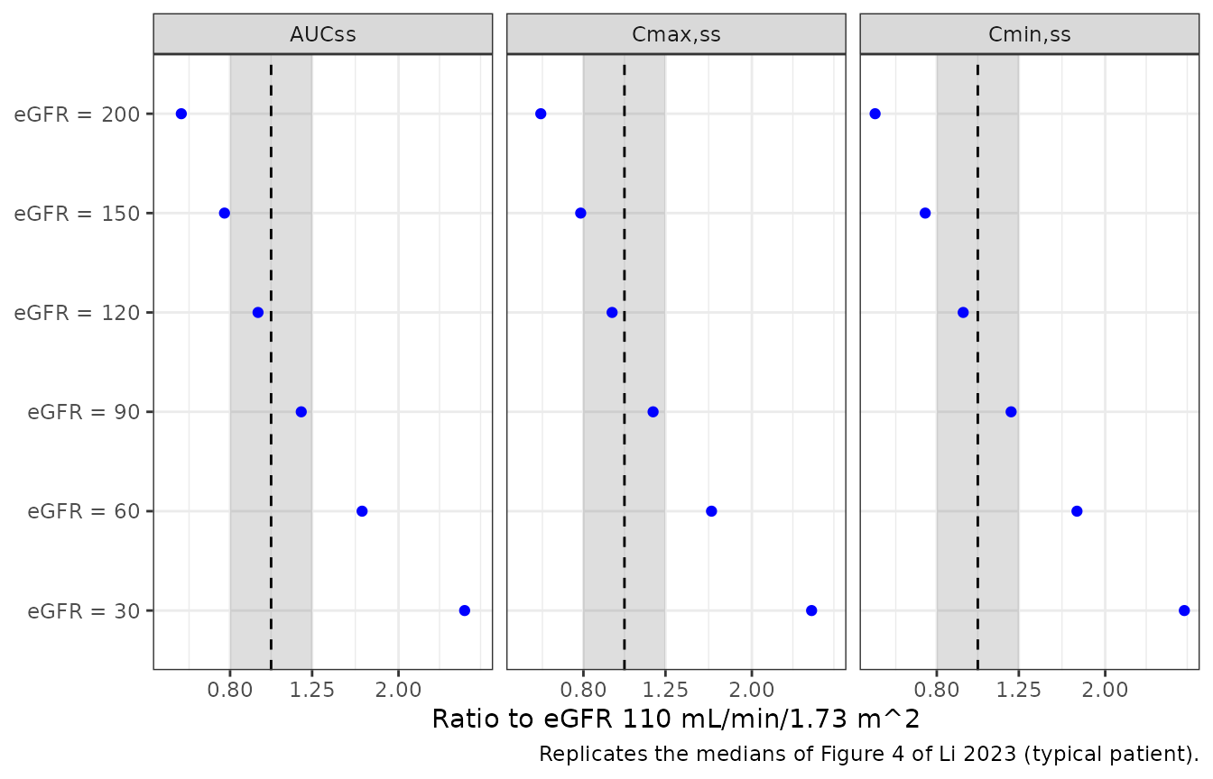
TDM cohort check
Li 2023 Table 1 reports the development-cohort amisulpride concentration normalised by daily dose: median 0.67 ng/mL per mg (IQR 0.428-0.946). A virtual TDM cohort is built from the Table 1 covariate summaries and sampled once per subject at a random time within a twice-daily dosing interval after two weeks of dosing, with residual error included:
- eGFR log-normal with median 114 and the log-scale SD implied by the IQR 101-130, truncated to 40-200 mL/min/1.73 m^2;
- daily dose normal with mean 566 and SD 264 mg (Table 1), truncated to the 100-1190 mg range of the development cohort and rounded to 50 mg, split into two equal doses (the per-patient regimen is not reported).
The same cohort is solved under both IIV readings from the IIV scale section.
set.seed(20230916)
n_tdm <- 200L
egfr_sdlog <- (log(130) - log(101)) / (2 * qnorm(0.75))
subj_tdm <- tibble::tibble(
  id = seq_len(n_tdm),
  CRCL = pmin(pmax(114 * exp(rnorm(n_tdm, 0, egfr_sdlog)), 40), 200),
  daily = round(pmin(pmax(rnorm(n_tdm, 566, 264), 100), 1190) / 50) * 50,
  t_obs = 336 + runif(n_tdm, 0, 12)
) |>
  mutate(
    dose_am = daily / 2, dose_pm = daily / 2,
    regimen = "TDM", egfr_label = "TDM"
  )

# Doses to 336 h, then one observation per subject at its own time.
ev_tdm <- bind_rows(
  make_events(subj_tdm, numeric(0), last_dose = 336),
  subj_tdm |>
    transmute(
      id, time = t_obs, amt = NA_real_, evid = 0L, cmt = "central",
      CRCL, regimen, egfr_label
    )
) |>
  arrange(id, time, desc(evid))

# omega^2 = CV^2: 0.359^2 and 1.309^2
mod_alt <- mod |>
  rxode2::ini(etalcl ~ 0.128881, etalvc ~ 1.713481)
#> ℹ parameter labels from comments will be replaced by 'label()'
#> ℹ change initial estimate of `etalcl` to `0.128881`
#> ℹ change initial estimate of `etalvc` to `1.713481`

solve_tdm <- function(m, seed) {
  rxode2::rxSetSeed(seed)
  rxode2::rxSolve(m, events = ev_tdm) |>
    as.data.frame() |>
    filter(!is.na(Cc)) |>
    select(id, sim) |>
    left_join(select(subj_tdm, id, daily), by = "id") |>
    mutate(cd = sim / daily)
}
tdm_pack <- solve_tdm(mod, 20230917)
tdm_alt <- solve_tdm(mod_alt, 20230917)

tdm_sum <- bind_rows(
  tibble::tibble(source = "Li 2023 Table 1 (observed)", q25 = 0.428, q50 = 0.67, q75 = 0.946),
  tdm_pack |> summarise(q25 = quantile(cd, 0.25), q50 = median(cd), q75 = quantile(cd, 0.75)) |>
    mutate(source = "Simulated, omega^2 = log(1 + CV^2) (packaged)"),
  tdm_alt |> summarise(q25 = quantile(cd, 0.25), q50 = median(cd), q75 = quantile(cd, 0.75)) |>
    mutate(source = "Simulated, omega^2 = CV^2")
) |>
  select(source, q25, q50, q75)

tdm_sum |>
  dplyr::rename(
    "Source" = source,
    "25th percentile" = q25,
    "Median" = q50,
    "75th percentile" = q75
  ) |>
knitr::kable(digits = 3, caption = "Dose-normalised concentration (ng/mL per mg daily dose).")| Source | 25th percentile | Median | 75th percentile |
|---|---|---|---|
| Li 2023 Table 1 (observed) | 0.428 | 0.670 | 0.946 |
| Simulated, omega^2 = log(1 + CV^2) (packaged) | 0.502 | 0.682 | 0.930 |
| Simulated, omega^2 = CV^2 | 0.499 | 0.675 | 0.930 |
stopifnot(
  # The centre is set by CL/F alone (1000 / (24 * 60.5) = 0.69 at the
  # reference eGFR); a wrong CL/F, unit or exponent moves it by tens of percent.
  abs(tdm_sum$q50[2] / 0.67 - 1) < 0.15
)
The simulated median matches the observed 0.67 ng/mL per mg. The simulated IQR is a little narrower at the lower end than the observed one, which is expected given that the virtual cohort has no once-daily or unequal split regimens and no non-adherence. The two IIV readings give nearly the same distribution, which is why this check cannot choose between them.
Assumptions and deviations
-
IIV scale. Table 2 reports IIV as %CV only. The
maintainers converted with
omega^2 = log(1 + CV^2); the alternativeomega^2 = CV^2gives a V/F variance of 1.71 instead of 1.00. See The IIV scale. -
No IIV on Ka. The control stream (Supplementary
Figure S6) carries an
ETA(3)on Ka with variance0 FIX, i.e. no variability; it is omitted. - Centring value. The eGFR reference is 113.84 mL/min/1.73 m^2 as printed in the Table 2 equation and the control stream. (A later summary of this model in Yan 2024, doi:10.2147/DDDT.S469149, prints 113.87.)
- Figure 6 dosing. The simulation follows the R code of Supplementary Figure S7 (morning dose at 0 h and evening dose at 12 h, every 24 h, plotted over 144-168 h). That code samples no random effects, but Figure 6 shows percentile bands, so IIV on CL/F and V/F and residual error are sampled here (the band-width table above shows why residual error is included). The paper simulated 500 subjects per regimen; 100 per regimen and eGFR level are used here.
- Results 3.5 versus Figure 6. The text states that at 1200 mg/day “all patients regardless of their renal function would have exceeded the laboratory alert threshold”, but in Figure 6C (eGFR 200) the 600 mg + 600 mg median lies below 640 ng/mL, as it does here (typical Cav about 520 ng/mL). The figure is consistent with the model; the sentence is not checked.
- Virtual TDM cohort. The per-patient dose regimen, sampling times and eGFR distribution are not published; the cohort above is built from the Table 1 summaries with the stated assumptions (twice-daily equal doses, random sampling time, log-normal eGFR).
- Table 1 inconsistencies. The Table 1 dose range columns (development 100-1190 mg, validation 50-1220 mg) are swapped relative to Results 3.1 (development 50-1220 mg, validation 100-1190 mg), and the Results text gives the validation cohort as 38.8% female while Table 1 gives 47.6%. Neither affects the model.
- No correction notice for Li 2023 was found (literature check 2026-10-27).