Evobrutinib (Papasouliotis 2022)
Source:vignettes/articles/Papasouliotis_2022_evobrutinib.Rmd
Papasouliotis_2022_evobrutinib.RmdModel and source
- Citation: Papasouliotis O, Mitchell D, Girard P, Dyroff M. Population pharmacokinetic and pharmacodynamic modeling of evobrutinib in healthy adult participants. Clin Transl Sci. 2022;15(12):2899-2908. doi:10.1111/cts.13417
- Description: Two-compartment population PK model with sequential zero-order (into the depot) then first-order absorption, absorption lag time and first-order elimination for oral evobrutinib tablets in healthy adults, with a food effect on bioavailability (+49%) and on the zero-order input duration (+427%), linked to an irreversible-binding turnover model of the fraction of unoccupied Bruton’s tyrosine kinase (BTK) in peripheral blood mononuclear cells
- Article: https://doi.org/10.1111/cts.13417 (open access)
Evobrutinib is an oral, covalent (irreversible) inhibitor of Bruton’s
tyrosine kinase (BTK). Papasouliotis 2022 fitted a population PK model
to plasma concentrations from two phase I studies in healthy adults and
a population PD model to BTK occupancy (BTKO) measured in peripheral
blood mononuclear cells, then combined the two to simulate steady-state
BTKO under alternative once-daily (q.d.) and twice-daily (b.i.d.)
regimens. The PK and BTKO models were estimated sequentially but are
used jointly for simulation, so they are packaged here as one model with
two endpoints: Cc (evobrutinib plasma concentration, ng/mL)
and target (fraction of unoccupied BTK relative to
predose). The derived output btko = 1 - target is the
occupied fraction.
Population
The PK analysis pooled 76 healthy adult participants (2326 plasma observations, 29% below the 0.600 ng/mL LLOQ and handled with the M3 method):
- Study MS200527_0017 Part A (n = 42; 7 Japanese and 7 non-Japanese per cohort): evobrutinib 25, 75 or 200 mg q.d. tablets for 6 days, fasted.
- Study MS200527_0017 Part B (n = 16; 8 Japanese, 8 non-Japanese): single 75 mg dose fed (low-fat meal) and fasted, two-period crossover.
- Study MS200527_0019 (n = 18): single 75 mg tablet dose fed (low-fat meal) and fasted, crossover.
The BTKO model used 441 observations from 41 Part A participants (14,
13 and 14 at 25, 75 and 200 mg). Baseline demographics (age, weight,
sex) are not tabulated in the paper; sex, weight, BMI, BSA, Japanese
ethnicity, age and dose were tested as covariates and none was retained.
The only covariate in the final model is prandial state. See
Papasouliotis 2022 Methods “Study population” and Table 1. The same
information is available programmatically via
readModelDb("Papasouliotis_2022_evobrutinib")()$population.
Source trace
Every ini() value carries an in-file comment pointing to
its source in
inst/modeldb/specificDrugs/Papasouliotis_2022_evobrutinib.R;
the table below collects them.
| Equation / parameter | Value | Source location |
|---|---|---|
lcl (CL/F) |
log(273 L/h) | Table 2 |
lvc (V2/F) |
log(61.1 L) | Table 2 |
lq (Q/F) |
log(37 L/h) | Table 2 |
lvp (V3/F) |
log(446 L) | Table 2 |
lka (Ka) |
log(0.784 1/h) | Table 2 |
ltlag (ALAG) |
log(0.235 h) | Table 2 |
ld1 (D1, fasted) |
log(0.181 h) | Table 2 |
e_fed_fdepot (Food on F1) |
1.49 | Table 2; Results “increased by 49%” |
e_fed_d1 (Food on D1) |
4.27, D1 x (1 + 4.27) | Table 2 and its footnote (D1 fed = 0.954 h) |
etalcl, etaltlag, covariance |
0.0958, 0.156, 0.0558 | Table 2 |
etalq, etalvp, covariance |
1.17, 1.86, 0.988 | Table 2 |
etalvc |
0.627 | Table 2 |
etald1_fasted, etald1_fed
|
1.39 each | Table 2 (“BPV D1 Fasted”, “BPV D1 Fed”) |
addSd, propSd (PK) |
0.214 ng/mL, 0.49 | Table 2; Results “49%” |
lkout (kout) |
log(0.00437 1/h) | Table 3; Results recovery half-life 159 h |
lkirrev (kirrev) |
log(0.0135 mL/ng/h) | Table 3 |
etalkout, etalkirrev
|
0.217, 0.103 | Table 3 |
addSd_target, propSd_target
|
0.00317, 0.43 | Table 3 |
| Absorption: dose -> zero-order (D1) into depot after ALAG -> Ka -> central | n/a | Figure 1; Methods “sequential zero-first order absorption” |
| Two-compartment disposition, first-order elimination | n/a | Figure 1 |
d/dt(target) = kin - kout*target - kirrev*Cc*target |
n/a | Methods, BTKO model equation |
kin = kout (BTK_FU,0 = 1) |
n/a | Methods, steady-state equation and text |
Virtual cohorts
mod <- readModelDb("Papasouliotis_2022_evobrutinib")

# rxSetSeed() fixes rxode2's random stream per solver thread but not across
# thread counts, so every assertion below is written to hold for any cohort.
rxode2::rxSetSeed(20221213)

# One cohort = `n` subjects given `ndose` doses every `ii` hours, all records
# sharing one prandial state. Doses use rate = -2 so rxode2 applies the
# modelled zero-order input duration dur(depot). Observation rows sit on the
# `target` state (an ODE state that is also a declared endpoint); rxode2
# returns Cc and btko on every row.
make_cohort <- function(n, dose, fed, ndose, ii, obs_times, label, id_offset) {
  ids <- id_offset + seq_len(n)
  dosing <- tidyr::crossing(id = ids, time = seq(0, by = ii, length.out = ndose)) |>
    mutate(amt = dose, evid = 1L, cmt = "depot", rate = -2)
  obs <- tidyr::crossing(id = ids, time = obs_times) |>
    mutate(amt = NA_real_, evid = 0L, cmt = "target", rate = NA_real_)
  bind_rows(dosing, obs) |>
    mutate(FED = fed, treatment = label) |>
    arrange(id, time, desc(evid)) |>
    select(id, time, amt, evid, cmt, rate, FED, treatment)
}
Figure 2 cohorts (study design)
Part A: 25, 75 and 200 mg q.d. for 6 days, fasted, with dense PK on Days 1 and 6 and BTKO sampled through Day 12. Part B / Study 0019: a single 75 mg dose with a low-fat meal.
n_arm <- 100
obs_partA <- sort(unique(c(seq(0, 24, by = 0.25), seq(120, 144, by = 0.25), seq(144, 264, by = 4))))
events_fig2 <- bind_rows(
  make_cohort(n_arm, 25, 0, 6, 24, obs_partA, "25 mg q.d. fasted", 0L),
  make_cohort(n_arm, 75, 0, 6, 24, obs_partA, "75 mg q.d. fasted", n_arm),
  make_cohort(n_arm, 200, 0, 6, 24, obs_partA, "200 mg q.d. fasted", 2L * n_arm),
  make_cohort(n_arm, 75, 1, 1, 24, seq(0, 48, by = 0.25), "75 mg single dose fed", 3L * n_arm)
)
stopifnot(!anyDuplicated(unique(events_fig2[, c("id", "time", "evid")])))Replicate published figures
Figure 2: concentration-time profiles on Days 1 and 6
sim_fig2 |>
  filter(time <= 24 | (time >= 120 & time <= 144 & treatment != "75 mg single dose fed")) |>
  mutate(
    day = ifelse(time <= 24, "Day 1", "Day 6"),
    tday = ifelse(time <= 24, time, time - 120)
  ) |>
  group_by(treatment, day, tday) |>
  summarise(
    Q05 = quantile(Cc, 0.05), Q50 = median(Cc), Q95 = quantile(Cc, 0.95),
    .groups = "drop"
  ) |>
  ggplot(aes(tday, Q50)) +
  geom_ribbon(aes(ymin = Q05, ymax = Q95), alpha = 0.25) +
  geom_line() +
  geom_hline(yintercept = 0.6, linetype = "dashed") +
  facet_grid(day ~ treatment) +
  scale_y_log10(limits = c(0.05, 2000)) +
  labs(
    x = "Time after dose (h)", y = "Evobrutinib concentration (ng/mL)",
    title = "Simulated median and 90% interval; dashed line = LLOQ 0.6 ng/mL",
    caption = "Replicates Figure 2 of Papasouliotis 2022."
  )
#> Warning in scale_y_log10(limits = c(0.05, 2000)): log-10 transformation introduced infinite values.
#> log-10 transformation introduced infinite values.
#> log-10 transformation introduced infinite values.
#> log-10 transformation introduced infinite values.
#> Warning: Removed 196 rows containing missing values or values outside the scale range
#> (`geom_ribbon()`).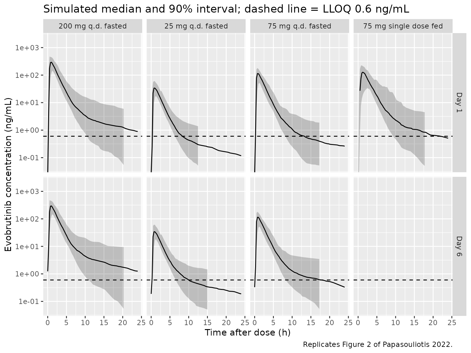
The simulated medians reach about 30-50 ng/mL at 25 mg, 100-150 ng/mL at 75 mg and several hundred ng/mL at 200 mg within 1 h, and fall below the LLOQ by 12-24 h at 25 and 75 mg, as in Figure 2 of the paper. There is little accumulation between Day 1 and Day 6, consistent with the short effective half-life.
BTK occupancy through Day 12 (Part A design)
sim_fig2 |>
  filter(treatment != "75 mg single dose fed") |>
  group_by(treatment, time) |>
  summarise(
    Q05 = quantile(btko, 0.05), Q50 = median(btko), Q95 = quantile(btko, 0.95),
    .groups = "drop"
  ) |>
  ggplot(aes(time / 24, Q50, colour = treatment, fill = treatment)) +
  geom_ribbon(aes(ymin = Q05, ymax = Q95), alpha = 0.15, colour = NA) +
  geom_line() +
  labs(
    x = "Time after first dose (day)", y = "BTK occupancy (fraction)",
    title = "BTKO, 6 days of q.d. dosing then washout",
    caption = "Part A design (BTKO sampled to Day 12); the BTKO VPC itself is Figure S5 of Papasouliotis 2022."
  )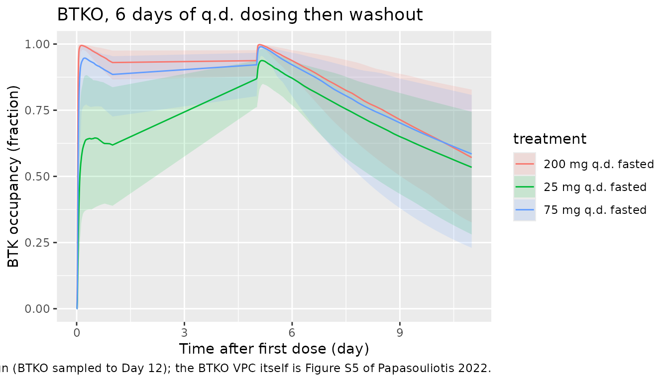
Table 4: steady-state minimum BTKO by regimen
The paper simulated 1000 participants per regimen for 14 days and
reported the percentage whose minimum BTKO over the last 24 h exceeded
70%, 80%, 90% and 95%, without residual error. The same design is
reproduced below with 200 participants per regimen (the package cap).
BTKO depends on the PK only through Cc, so only the typical
PK-PD linkage and the PK and PD random effects matter here.
n_t4 <- 200
doses <- c(25, 50, 75, 100, 200)
design_t4 <- tidyr::crossing(
  dose = doses, regimen = c("q.d.", "b.i.d."), fed = c(0, 1)
) |>
  mutate(k = row_number())
obs_ss <- seq(13 * 24, 14 * 24, by = 0.5)
events_t4 <- bind_rows(lapply(seq_len(nrow(design_t4)), function(i) {
  d <- design_t4[i, ]
  ii <- if (d$regimen == "q.d.") 24 else 12
  make_cohort(
    n_t4, d$dose, d$fed, 14 * 24 / ii, ii, obs_ss,
    paste(d$dose, d$regimen, d$fed), (d$k - 1L) * n_t4
  )
}))
stopifnot(!anyDuplicated(unique(events_t4[, c("id", "time", "evid")])))

sim_t4 <- rxode2::rxSolve(
  mod,
  events = events_t4,
  keep = c("treatment"),
  sigma = NA, # no residual error, as in the paper
  useLinCmt = FALSE,
  returnType = "data.frame"
)

min_btko <- sim_t4 |>
  group_by(treatment, id) |>
  summarise(min_btko = min(btko), .groups = "drop") |>
  tidyr::separate(treatment, c("dose", "regimen", "fed"), sep = " ") |>
  mutate(dose = as.numeric(dose), prandial = ifelse(fed == "1", "Fed", "Fasted"))

thresholds <- c(0.70, 0.80, 0.90, 0.95)
sim_pct <- tidyr::crossing(min_btko, threshold = thresholds) |>
  group_by(regimen, prandial, threshold, dose) |>
  summarise(sim = 100 * mean(min_btko >= threshold), .groups = "drop")

published_t4 <- tibble::tribble(
  ~regimen, ~prandial, ~threshold, ~`25`, ~`50`, ~`75`, ~`100`, ~`200`,
  "q.d.", "Fasted", 0.70, 98, 100, 100, 100, 100,
  "q.d.", "Fasted", 0.80, 88, 97, 99, 99, 100,
  "q.d.", "Fasted", 0.90, 36, 59, 71, 77, 87,
  "q.d.", "Fasted", 0.95, 4, 13, 20, 24, 39,
  "q.d.", "Fed", 0.70, 99, 100, 100, 100, 100,
  "q.d.", "Fed", 0.80, 95, 99, 99, 99, 100,
  "q.d.", "Fed", 0.90, 54, 74, 82, 85, 92,
  "q.d.", "Fed", 0.95, 10, 22, 29, 34, 51,
  "b.i.d.", "Fasted", 0.70, 100, 100, 100, 100, 100,
  "b.i.d.", "Fasted", 0.80, 99, 100, 100, 100, 100,
  "b.i.d.", "Fasted", 0.90, 88, 97, 99, 100, 100,
  "b.i.d.", "Fasted", 0.95, 38, 68, 81, 86, 94,
  "b.i.d.", "Fed", 0.70, 100, 100, 100, 100, 100,
  "b.i.d.", "Fed", 0.80, 100, 100, 100, 100, 100,
  "b.i.d.", "Fed", 0.90, 96, 99, 100, 100, 100,
  "b.i.d.", "Fed", 0.95, 59, 85, 90, 93, 97
) |>
  tidyr::pivot_longer(c(`25`, `50`, `75`, `100`, `200`), names_to = "dose", values_to = "published") |>
  mutate(dose = as.numeric(dose))

t4_cmp <- inner_join(published_t4, sim_pct, by = c("regimen", "prandial", "threshold", "dose")) |>
  mutate(diff = sim - published)
stopifnot(nrow(t4_cmp) == 80)

t4_cmp |>
  mutate(cell = sprintf("%.0f / %.0f", sim, published)) |>
  select(regimen, prandial, threshold, dose, cell) |>
  tidyr::pivot_wider(names_from = dose, values_from = cell) |>
  rename(
    "Regimen" = regimen, "Prandial state" = prandial, "BTKO threshold" = threshold,
    "25 mg" = `25`, "50 mg" = `50`, "75 mg" = `75`, "100 mg" = `100`, "200 mg" = `200`
  ) |>
knitr::kable(caption = "Percentage of participants with minimum steady-state BTKO above each threshold: simulated (n = 200 per regimen) / published (Table 4, n = 1000).")| Regimen | Prandial state | BTKO threshold | 25 mg | 50 mg | 75 mg | 100 mg | 200 mg |
|---|---|---|---|---|---|---|---|
| q.d. | Fasted | 0.70 | 99 / 98 | 100 / 100 | 100 / 100 | 100 / 100 | 100 / 100 |
| q.d. | Fasted | 0.80 | 90 / 88 | 94 / 97 | 98 / 99 | 98 / 99 | 100 / 100 |
| q.d. | Fasted | 0.90 | 38 / 36 | 59 / 59 | 70 / 71 | 76 / 77 | 85 / 87 |
| q.d. | Fasted | 0.95 | 6 / 4 | 11 / 13 | 20 / 20 | 27 / 24 | 34 / 39 |
| q.d. | Fed | 0.70 | 100 / 99 | 100 / 100 | 100 / 100 | 100 / 100 | 100 / 100 |
| q.d. | Fed | 0.80 | 94 / 95 | 100 / 99 | 100 / 99 | 99 / 99 | 100 / 100 |
| q.d. | Fed | 0.90 | 56 / 54 | 73 / 74 | 76 / 82 | 78 / 85 | 88 / 92 |
| q.d. | Fed | 0.95 | 10 / 10 | 21 / 22 | 26 / 29 | 32 / 34 | 46 / 51 |
| b.i.d. | Fasted | 0.70 | 99 / 100 | 100 / 100 | 100 / 100 | 100 / 100 | 100 / 100 |
| b.i.d. | Fasted | 0.80 | 98 / 99 | 100 / 100 | 100 / 100 | 100 / 100 | 100 / 100 |
| b.i.d. | Fasted | 0.90 | 84 / 88 | 96 / 97 | 98 / 99 | 99 / 100 | 100 / 100 |
| b.i.d. | Fasted | 0.95 | 34 / 38 | 72 / 68 | 80 / 81 | 86 / 86 | 94 / 94 |
| b.i.d. | Fed | 0.70 | 100 / 100 | 100 / 100 | 100 / 100 | 100 / 100 | 100 / 100 |
| b.i.d. | Fed | 0.80 | 100 / 100 | 100 / 100 | 100 / 100 | 100 / 100 | 100 / 100 |
| b.i.d. | Fed | 0.90 | 98 / 96 | 100 / 99 | 100 / 100 | 100 / 100 | 100 / 100 |
| b.i.d. | Fed | 0.95 | 64 / 59 | 82 / 85 | 84 / 90 | 92 / 93 | 98 / 97 |
# Structural gate: a mis-transcribed kout, kirrev, CL/F or food effect moves
# whole rows of Table 4 by tens of percentage points. The cells near 0% or
# 100% carry little information, so the check is on the centre and a robust
# upper quantile of the absolute differences. With 200 subjects per regimen
# the binomial SE of a mid-range cell is about 3.5 percentage points.
t4_summary <- c(
  median_abs_diff = median(abs(t4_cmp$diff)),
  q90_abs_diff = unname(quantile(abs(t4_cmp$diff), 0.9)),
  max_abs_diff = max(abs(t4_cmp$diff))
)
t4_summary
#> median_abs_diff    q90_abs_diff    max_abs_diff
#>            0.50            3.55            6.50
stopifnot(
  t4_summary[["median_abs_diff"]] < 5,
  t4_summary[["q90_abs_diff"]] < 15
)
Across the 80 cells of Table 4 the median absolute difference between the simulated and published percentages is 0.5 percentage points and the 90th percentile is 3.6. The remaining differences are expected: the paper’s simulation also included five correlations of at least 30% between PK and BTKO random effects (largest 42%) whose values are not reported, and its cohorts were five times larger.
PKNCA validation
PKNCA on the Figure 2 cohorts: Day 1 (0-24 h) for every arm and the dosing interval on Day 6 for the q.d. arms.
sim_nca <- sim_fig2 |>
  filter(!is.na(Cc), time <= 144) |>
  select(id, time, Cc, treatment)
sim_nca <- bind_rows(
  sim_nca,
  sim_nca |> distinct(id, treatment) |> mutate(time = 0, Cc = 0)
) |>
  distinct(id, treatment, time, .keep_all = TRUE) |>
  arrange(id, treatment, time)

conc_obj <- PKNCA::PKNCAconc(sim_nca, Cc ~ time | treatment + id)
dose_df <- events_fig2 |>
  filter(evid == 1) |>
  select(id, time, amt, treatment)
dose_obj <- PKNCA::PKNCAdose(dose_df, amt ~ time | treatment + id)

# Every interval row names its treatment: the single-dose fed arm has no Day 6.
qd_arms <- c("25 mg q.d. fasted", "75 mg q.d. fasted", "200 mg q.d. fasted")
intervals <- bind_rows(
  data.frame(treatment = c(qd_arms, "75 mg single dose fed"), start = 0, end = 24),
  data.frame(treatment = qd_arms, start = 120, end = 144)
) |>
  mutate(cmax = TRUE, tmax = TRUE, auclast = TRUE)
nca_res <- PKNCA::pk.nca(PKNCA::PKNCAdata(conc_obj, dose_obj, intervals = intervals))

nca_tbl <- as.data.frame(nca_res$result) |>
  filter(PPTESTCD %in% c("cmax", "tmax", "auclast")) |>
  group_by(treatment, start, PPTESTCD) |>
  summarise(median = median(PPORRES, na.rm = TRUE), .groups = "drop") |>
  tidyr::pivot_wider(names_from = PPTESTCD, values_from = median)

nca_tbl |>
  mutate(
    interval = ifelse(start == 0, "Day 1 (0-24 h)", "Day 6 (120-144 h)"),
    across(c(cmax, tmax, auclast), \(x) signif(x, 3))
  ) |>
  select(treatment, interval, cmax, tmax, auclast) |>
  rename(
    "Treatment" = treatment, "Interval" = interval,
    "Cmax (ng/mL)" = cmax, "Tmax (h)" = tmax, "AUC0-24 (ng*h/mL)" = auclast
  ) |>
knitr::kable(caption = "Median simulated NCA parameters (n = 100 per arm).")| Treatment | Interval | Cmax (ng/mL) | Tmax (h) | AUC0-24 (ng*h/mL) |
|---|---|---|---|---|
| 200 mg q.d. fasted | Day 1 (0-24 h) | 325.0 | 0.875 | 732.0 |
| 200 mg q.d. fasted | Day 6 (120-144 h) | 327.0 | 0.875 | 785.0 |
| 25 mg q.d. fasted | Day 1 (0-24 h) | 37.4 | 0.750 | 84.7 |
| 25 mg q.d. fasted | Day 6 (120-144 h) | 37.6 | 0.750 | 88.5 |
| 75 mg q.d. fasted | Day 1 (0-24 h) | 124.0 | 0.750 | 277.0 |
| 75 mg q.d. fasted | Day 6 (120-144 h) | 126.0 | 0.750 | 283.0 |
| 75 mg single dose fed | Day 1 (0-24 h) | 153.0 | 1.500 | 383.0 |
Comparison against published NCA
Papasouliotis 2022 reports no NCA table. The closed form for a linear model is that AUC from zero to infinity after a single oral dose equals F x Dose / (CL/F), so for the typical participant it must be 75 / 273 x 1000 = 274.7 ng*h/mL fasted and 1.49 times that (409.3 ng*h/mL) fed. A typical-value solve analysed with PKNCA is compared against those closed-form values; this checks the structural model, the mg -> ng/mL scaling and the food effect on F together.
# 120 h captures > 99.99% of AUC; a longer window reaches ~1e-13 ng/mL
# integrator noise, which PKNCA turns into a NaN AUC.
ev_typ <- bind_rows(
  make_cohort(1, 75, 0, 1, 24, c(seq(0, 24, by = 0.1), seq(25, 120, by = 1)), "75 mg fasted", 0L),
  make_cohort(1, 75, 1, 1, 24, c(seq(0, 24, by = 0.1), seq(25, 120, by = 1)), "75 mg fed", 1L)
)
sim_typ <- rxode2::rxSolve(
  mod,
  events = ev_typ, keep = c("treatment"),
  omega = NA, sigma = NA, useLinCmt = FALSE,
  atol = 1e-10, rtol = 1e-10, returnType = "data.frame"
)
typ_conc <- PKNCA::PKNCAconc(
  bind_rows(
    sim_typ |> select(id, time, Cc, treatment),
    sim_typ |> distinct(id, treatment) |> mutate(time = 0, Cc = 0)
  ) |> distinct(id, treatment, time, .keep_all = TRUE) |> arrange(id, time),
  Cc ~ time | treatment + id
)
typ_dose <- PKNCA::PKNCAdose(
  ev_typ |> filter(evid == 1) |> select(id, time, amt, treatment),
  amt ~ time | treatment + id
)
typ_nca <- PKNCA::pk.nca(PKNCA::PKNCAdata(
  typ_conc, typ_dose,
  intervals = data.frame(start = 0, end = Inf, aucinf.obs = TRUE, cmax = TRUE)
))

closed_form <- tibble::tibble(
  treatment = c("75 mg fasted", "75 mg fed"),
  aucinf.obs = 1000 * 75 * c(1, 1.49) / 273
)
cmp <- nlmixr2lib::ncaComparisonTable(
  simulated = typ_nca,
  reference = closed_form,
  by = "treatment",
  params = "aucinf.obs",
  units = c(aucinf.obs = "ng*h/mL"),
  tolerance_pct = 20
)
knitr::kable(cmp, caption = "Typical-value PKNCA AUC0-inf vs. the closed form F x Dose / (CL/F). * differs by >20%.")| NCA parameter | treatment | Reference | Simulated | % diff |
|---|---|---|---|---|
| AUC0-∞ (obs) (ng*h/mL) | 75 mg fasted | 275 | 275 | -0.0% |
| AUC0-∞ (obs) (ng*h/mL) | 75 mg fed | 409 | 409 | -0.0% |
typ_auc <- as.data.frame(typ_nca$result) |>
  filter(PPTESTCD == "aucinf.obs") |>
  left_join(closed_form, by = "treatment")
# Same drawn parameters on both sides (typical values): the only difference is
# trapezoidal and extrapolation error, so a tight bound is correct.
stopifnot(all(abs(typ_auc$PPORRES / typ_auc$aucinf.obs - 1) < 0.02))
BTK recovery half-life
The paper states that the irreversible binding model estimates a BTK
recovery half-life of 159 h. After the drug has washed out,
d(target)/dt = kout * (1 - target), so occupancy decays as
exp(-kout * t). The typical-value washout slope after the
200 mg single dose reproduces it.
ev_rec <- make_cohort(1, 200, 0, 1, 24, seq(0, 720, by = 4), "200 mg", 0L)
sim_rec <- rxode2::rxSolve(
  mod,
  events = ev_rec, omega = NA, sigma = NA, useLinCmt = FALSE,
  returnType = "data.frame"
)
wash <- sim_rec |> filter(time >= 240, time <= 720)
fit <- lm(log(btko) ~ time, data = wash)
t_half_rec <- log(2) / -coef(fit)[["time"]]
t_half_rec
#> [1] 158.6149
stopifnot(abs(t_half_rec - 159) < 2)
Assumptions and deviations
- PK-PD random-effect correlations not included. The paper’s steady-state simulations used five correlations of at least 30% (largest 42%) between PK and BTKO random effects, but their values and the parameter pairs are not reported. The packaged model treats the PK and BTKO etas as independent, which is the most likely source of the residual differences from Table 4.
-
koutunits. Table 3 prints the unit ofkoutas “L/h”; it is a first-order rate constant (1/h), as confirmed by the stated recovery half-life of 159 h (ln 2 / 0.00437 = 158.6 h). - Residual error scale. Tables 2 and 3 report the additive and proportional residual errors without stating whether they are standard deviations or variances. They are encoded as standard deviations: the Results describe the proportional errors as 49% and 43%, and the PK additive term (0.214 ng/mL) is of the right size relative to the 0.600 ng/mL LLOQ.
-
Separate D1 etas per prandial state. The model
carried a distinct random effect on D1 for fed and fasted dosing within
the same participant; Table 2 reports the same variance (1.39) for both,
encoded as two etas with that variance, selected by
FED. -
Food effects. Bioavailability is 1 fasted and 1.49
fed (
e_fed_fdepot^FED); D1 is 0.181 h fasted and 0.181 x (1 + 4.27) = 0.954 h fed, as stated in the Table 2 footnote. All fed data came from a low-fat meal; the paper describes the covariate generically as food state, so the generalFEDindicator is used. -
BTKO baseline. BTK occupancy data were
baseline-corrected, so the fraction unoccupied starts at 1 and
kin = kout(Methods). The observed endpoint is the fraction unoccupied (target);btko = 1 - target. -
Covariate screen. Sex, weight, BMI, BSA, Japanese
versus non-Japanese ethnicity, age and dose were tested and not
retained; they are listed in
covariatesDataExcluded. - Cohort sizes. Figure 2 cohorts use 100 participants per arm and the Table 4 replication 200 per regimen (the paper used 1000).
- Demographics (age, weight, sex) are not reported, so the virtual cohorts carry no demographic covariates; none enters the model.
- No erratum or correction notice for this article was found as of 2026-10-10.