Triheptanoin / heptanoate (Lee 2022)
Source:vignettes/articles/Lee_2022_triheptanoin.Rmd
Lee_2022_triheptanoin.RmdModel and source
Triheptanoin is a medium-chain triglyceride of three seven-carbon fatty acids. Pancreatic lipases hydrolyse it in the gut, so almost none reaches the circulation intact; heptanoate is the most abundant and pharmacologically active metabolite in plasma. Lee 2022 fitted a population PK model of plasma heptanoate after oral triheptanoin in healthy adults and in pediatric and adult patients with long-chain fatty acid oxidation disorders (LC-FAOD), using Phoenix NLME (FOCE with interaction).
mod <- readModelDb("Lee_2022_triheptanoin")- Citation: Lee SK, Gosselin NH, Jomphe C, McKeever K, Putnam W. Population Pharmacokinetics of Heptanoate in Healthy Subjects and Patients With Long-Chain Fatty Acid Oxidation Disorders Treated With Triheptanoin. Clin Pharmacol Drug Dev. 2022;11(11):1264-1272. doi:10.1002/cpdd.1145. Final estimates from Table 3; bootstrap results and simulated exposures from Supplementary Tables S3 and S4.
- Article: https://doi.org/10.1002/cpdd.1145 (open access; PMC9795984)
- Supplement: Supplementary Tables S1-S4 and Figures S1-S2
(
CPDD-11-1264-s001.docx, distributed with the article).
One-compartment population PK model for heptanoate, the main circulating metabolite of oral triheptanoin, in healthy adults and in pediatric and adult patients with long-chain fatty acid oxidation disorders (LC-FAOD) (Lee 2022). Each triheptanoin dose is split between two parallel first-order absorption compartments: depot (typical 56.2 percent, ka1 0.425 1/h) and depot2 (43.8 percent, ka2 0.507 1/h, lag 3.74 h). Apparent clearance and volume scale allometrically with time-varying body weight (reference 58 kg); clearance is 19 percent lower in LC-FAOD patients than in healthy subjects and falls with time since the first dose by up to 45 percent (T50 86.7 h). Doses are entered as umol triheptanoin; each mole releases three moles of heptanoate.
Population
The analysis pooled 562 measurable heptanoate concentrations from 43 subject IDs in three studies (Supplementary Tables S1 and S2): a phase 1 crossover study in 13 healthy adults who took triheptanoin oil at 1.25 or 1.5 g/kg/day, a phase 2 study in patients with LC-FAOD, and the PK sub-study of its long-term extension. Patients took triheptanoin with food or by gastrostomy tube at least four times a day, at 25-35 percent of daily caloric intake. Two patients took part in two studies and were given separate IDs.
Of the 30 LC-FAOD subjects, 23 were children or adolescents (five infants aged 6 months to under 2 years, 13 children aged 2 to under 12 years and five adolescents) and 7 were adults (Table 2). Mean body weight was 73.8 kg in the healthy adults, 35.0 kg in pediatric patients and 83.6 kg in adult patients (Table 1); the overall range was 8.23-121 kg with a median of 58 kg. Twenty of the 43 IDs (46.5 percent) were female and 35 (81.4 percent) were White.
str(rxode2::rxode2(mod)$population)
#> ℹ parameter labels from comments will be replaced by 'label()'
#> List of 14
#>  $ species       : chr "human"
#>  $ n_subjects    : num 43
#>  $ n_studies     : num 3
#>  $ age_range     : chr "0.87-62.1 years (LC-FAOD pediatric 0.87-17.9 y; LC-FAOD adult 19.2-62.1 y)"
#>  $ age_mean      : chr "healthy 39.1 y; LC-FAOD pediatric 7.41 y; LC-FAOD adult 33.6 y"
#>  $ weight_range  : chr "8.23-121 kg"
#>  $ weight_median : chr "58 kg (overall PK population)"
#>  $ sex_female_pct: num 46.5
#>  $ race_ethnicity: Named num [1:5] 81.4 9.3 2.3 2.3 4.7
#>   ..- attr(*, "names")= chr [1:5] "White" "Black" "Asian" "NativeHawaiianPacificIslander" ...
#>  $ disease_state : chr "13 healthy adults and 30 patients with long-chain fatty acid oxidation disorders (23 pediatric, 7 adult)"
#>  $ dose_range    : chr "Triheptanoin oil 1.25 or 1.5 g/kg/day orally in healthy subjects; 25-35 percent of daily caloric intake in at l"| __truncated__
#>  $ regions       : chr "not reported"
#>  $ n_observations: num 562
#>  $ notes         : chr "Table 1 (continuous) and Table 2 (categorical) baseline demographics; Supplementary Table S1 lists the three st"| __truncated__
Source trace
Every ini() value carries an in-file comment pointing to
its source. The table collects them.
| Equation / parameter | Value | Source location |
|---|---|---|
| Structure: 1-compartment, two parallel first-order absorption compartments, lag on the second | n/a | Figure 1; Results, Model Development |
lka (Ka1) |
0.425 1/h | Table 3 |
lka2 (Ka2) |
0.507 1/h | Table 3 |
ltlag2 (Lag2) |
3.74 h | Table 3 |
logitfrac (1 - F1) |
F1 = 0.562 | Table 3; logit form in Table 3 footnote b |
lcl (CL/F0, LC-FAOD) |
471 L/h | Table 3 |
e_healthy_cl |
584 / 471 | Table 3 (CL/F0 healthy = 584 L/h) |
e_wt_cl (Expo_CL) |
1.07 | Table 3 |
lcl_time_max (MAX) |
0.450 | Table 3 |
lcl_t50 (T50) |
86.7 h | Table 3 |
lvc (V/F0) |
5.56 L | Table 3 |
e_wt_vc (Expo_V) |
1.13 | Table 3 |
| CL/F equation | CL/F0 * (WT/58)^Expo_CL * (1 - MAX * TIME/(T50 + TIME)) |
Table 3 footnote c |
| V/F equation | V/F0 * (WT/58)^Expo_V |
Table 3 footnote d |
Factor 3 in f(depot), f(depot2)
|
3 mol heptanoate per mol triheptanoin | Table 3 footnote a; Methods (MW 428.61 g/mol) |
etalogitfrac |
1.09 (logit-scale variance) | Table 3 and footnote b |
etalka |
log(1 + 1.34^2) | Table 3: BSV Ka1 = 134 percent |
etalcl |
log(1 + 0.601^2) | Table 3: BSV CL/F = 60.1 percent |
expSd |
0.764 | Table 3: log-additive error |
Dosing in this model
Doses are entered in micromoles of triheptanoin: a
dose of D g/kg in a subject of WT kg is
D / 428.61 * 1e6 * WT umol. The model multiplies by three
inside f(), so the depots receive heptanoate. Each dose
needs two records with the same amount, one to depot and
one to depot2; f() then splits it F1 / (1 -
F1). Time t is the time since the first triheptanoin dose,
which the time-dependent decrease in CL/F is measured from.
mw_triheptanoin <- 428.61 # g/mol, Methods
dose_umol <- function(g_per_kg, wt) g_per_kg / mw_triheptanoin * 1e6 * wt

# Four doses a day with an 8-hour pause overnight (Methods, Model Application):
# the 16-hour day is split into three equal intervals of 16/3 h.
daily_dose_times <- c(0, 16 / 3, 32 / 3, 16)
n_days <- 7
dose_times <- as.vector(outer(daily_dose_times, 24 * (seq_len(n_days) - 1), `+`))
last_dose <- max(dose_times)
day7 <- 24 * (n_days - 1)

# Observation grid: every 0.25 h on day 7 and for 24 h after the last dose,
# plus the day-7 dose times so pre-dose troughs are recorded exactly.
obs_times <- sort(unique(c(
  seq(0, day7, by = 1),
  seq(day7, last_dose + 24, by = 0.25),
  day7 + daily_dose_times
)))
Virtual cohort
The paper’s exposure summary (Supplementary Table S4) simulates 1.25 g/kg/day (2916 umol/kg/day) given four times a day for each analysed subject, using their posterior Bayes parameters. The individual data are not available, so the cohort below draws subjects from the population model instead, with body weights matched to Table 1 (log-normal with the tabulated mean and CV; pediatric weights truncated to the observed 8.23-121 kg range).
set.seed(2022)
n_per_group <- 150

make_cohort <- function(n, group, wt_mean, wt_cv, healthy, id_offset) {
  sdlog <- sqrt(log(1 + wt_cv^2))
  wt <- wt_mean * exp(rnorm(n, -sdlog^2 / 2, sdlog))
  wt <- pmin(pmax(wt, 8.23), 121)
  subj <- tibble(id = id_offset + seq_len(n), WT = wt, DIS_HEALTHY = healthy, group = group)
  doses <- tidyr::crossing(subj, time = dose_times, cmt = c("depot", "depot2")) |>
    mutate(evid = 1L, amt = dose_umol(1.25 / 4, WT))
  obs <- tidyr::crossing(subj, time = obs_times) |>
    mutate(cmt = "central", evid = 0L, amt = 0)
  bind_rows(doses, obs)
}

events <- bind_rows(
  make_cohort(n_per_group, "Healthy adults", 73.8, 0.176, 1L, 0L),
  make_cohort(n_per_group, "LC-FAOD adults", 83.6, 0.242, 0L, n_per_group),
  make_cohort(n_per_group, "LC-FAOD pediatric", 35.0, 0.793, 0L, 2L * n_per_group)
) |>
  # observations before doses at the same time, so a pre-dose record is a trough
  arrange(id, time, evid) |>
  select(id, time, evid, amt, cmt, WT, DIS_HEALTHY, group)
stopifnot(!anyDuplicated(unique(events[, c("id", "time", "evid", "cmt")])))
Simulation
rxode2::rxSetSeed(2022)
sim <- rxode2::rxSolve(mod, events = events, keep = c("group", "WT")) |>
  as.data.frame()
#> ℹ parameter labels from comments will be replaced by 'label()'
Typical profiles over the first week
The time-dependent decrease in CL/F (up to 45 percent, T50 86.7 h) makes heptanoate accumulate over the first days of dosing. The figure shows the typical profile for a 58 kg subject.
typical_events <- bind_rows(
  tidyr::crossing(id = 1:2, time = dose_times, cmt = c("depot", "depot2")) |>
    mutate(evid = 1L, amt = dose_umol(1.25 / 4, 58)),
  tidyr::crossing(id = 1:2, time = seq(0, last_dose + 24, by = 0.05)) |>
    mutate(cmt = "central", evid = 0L, amt = 0)
) |>
  mutate(WT = 58, DIS_HEALTHY = ifelse(id == 1, 1L, 0L)) |>
  arrange(id, time, evid)
sim_typ <- rxode2::rxSolve(rxode2::zeroRe(mod), events = typical_events,
                           keep = "DIS_HEALTHY") |>
  as.data.frame() |>
  mutate(group = ifelse(DIS_HEALTHY == 1, "Healthy (58 kg)", "LC-FAOD (58 kg)"))
#> ℹ parameter labels from comments will be replaced by 'label()'
#> ℹ omega/sigma items treated as zero: 'etalogitfrac', 'etalka', 'etalcl'
#> Warning: multi-subject simulation without without 'omega'

ggplot(sim_typ, aes(time / 24, Cc, colour = group)) +
  geom_line(linewidth = 0.4) +
  labs(x = "Time since first dose (day)", y = "Heptanoate (umol/L)", colour = NULL,
       title = "Typical heptanoate profile, 1.25 g/kg/day triheptanoin in four doses") +
  theme(legend.position = "bottom")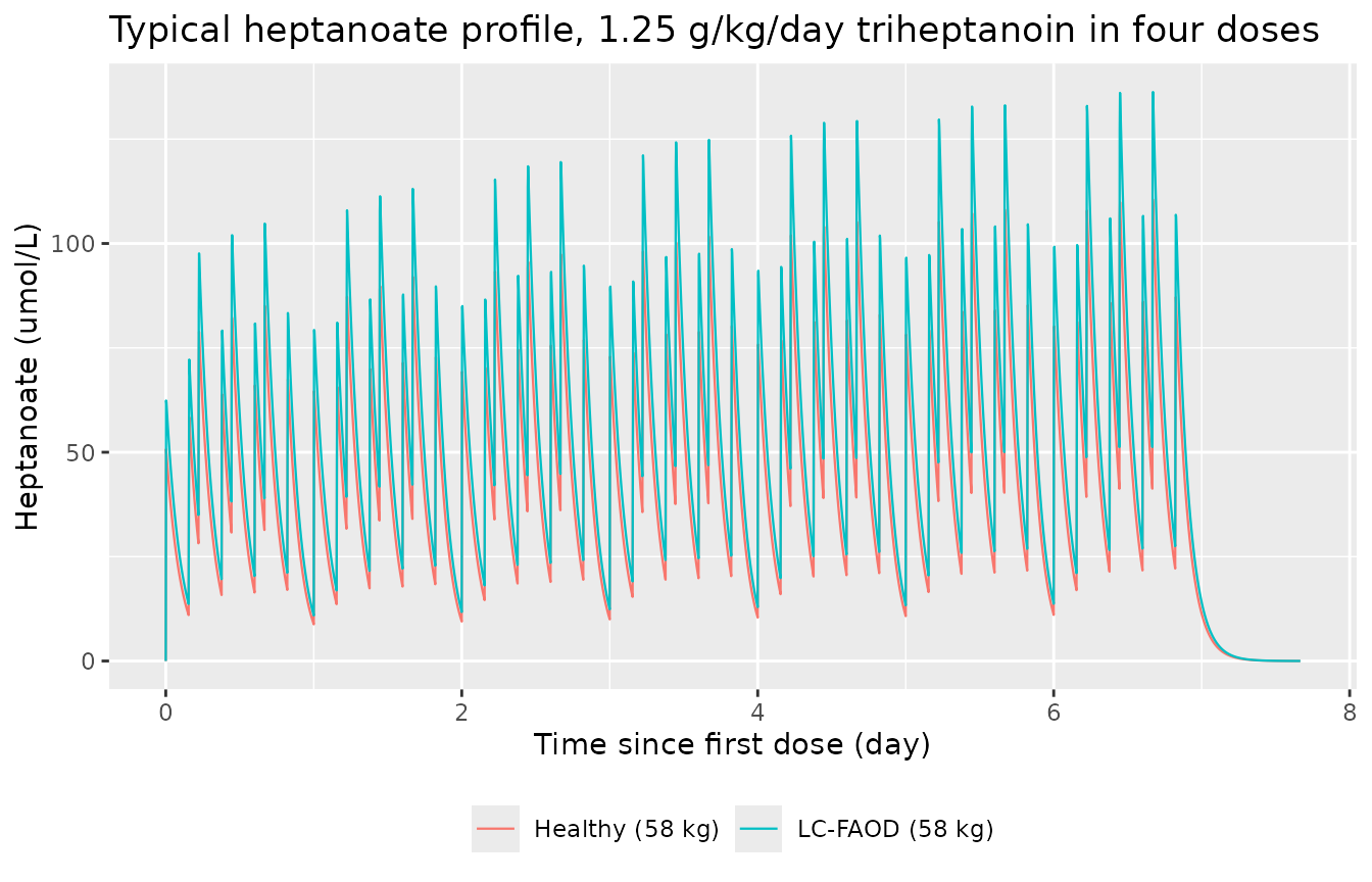
Day-7 concentration-time profile
The paper’s VPC (Supplementary Figure S2) pools the observed sampling times of each study, so it cannot be redrawn for a fixed regimen. The figure below shows the simulated median and 90 percent interval on day 7 of the four-times-daily regimen for each group.
sim |>
  filter(time >= day7, time <= day7 + 24) |>
  group_by(group, time) |>
  summarise(
    Q05 = quantile(Cc, 0.05), Q50 = median(Cc), Q95 = quantile(Cc, 0.95),
    .groups = "drop"
  ) |>
  ggplot(aes(time - day7, Q50)) +
  geom_ribbon(aes(ymin = Q05, ymax = Q95), alpha = 0.25) +
  geom_line() +
  facet_wrap(~group) +
  scale_y_log10() +
  labs(x = "Time on day 7 (h)", y = "Heptanoate (umol/L)",
       title = "Simulated day-7 profiles: median and 5th-95th percentiles")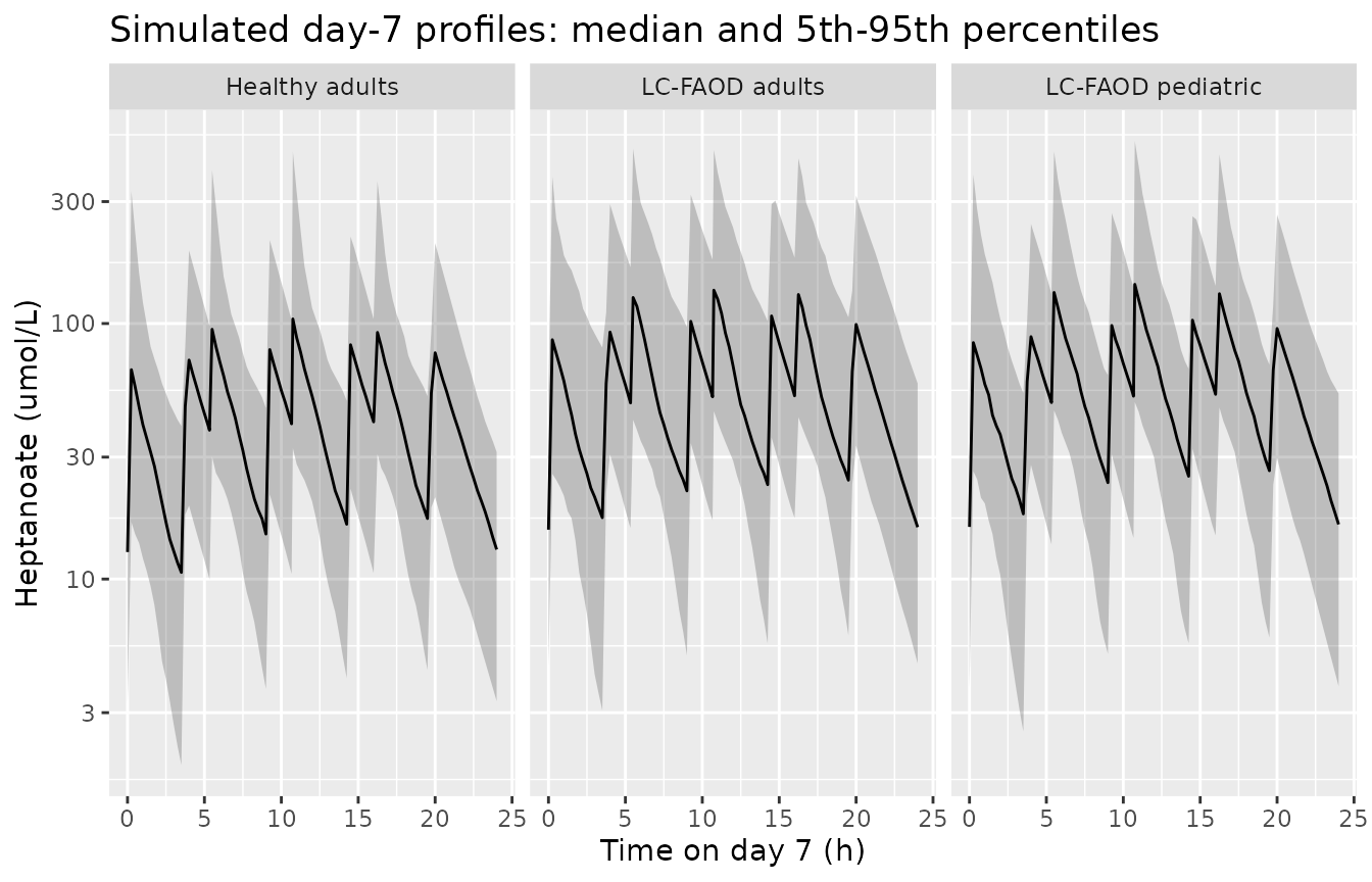
PKNCA validation
Supplementary Table S4 reports, per group, the daily AUC (AUCday), Cmax and Cmin at steady state, the time to Cmax and the terminal half-life after the last dose. The day the paper treats as steady state is not stated; because CL/F keeps falling with time, the comparison below uses day 7 (the healthy study ran 11 days and the patient studies weeks to months). AUCday, Cmax and Cmin are taken over day 7, Tmax over the first dosing interval of day 7, and the half-life from the 24 hours after the last dose.
sim_nca <- sim |>
  filter(!is.na(Cc)) |>
  select(id, time, Cc, group)
# Time-zero records anchor PKNCA; pre-dose heptanoate is zero.
sim_nca <- bind_rows(
  sim_nca,
  sim_nca |> distinct(id, group) |> mutate(time = 0, Cc = 0)
) |>
  distinct(id, group, time, .keep_all = TRUE) |>
  arrange(id, group, time)

dose_df <- events |>
  filter(evid == 1, cmt == "depot") |>
  select(id, time, amt, group)

conc_obj <- PKNCA::PKNCAconc(sim_nca, Cc ~ time | group + id)
dose_obj <- PKNCA::PKNCAdose(dose_df, amt ~ time | group + id)

intervals <- data.frame(
  start = c(day7, day7, last_dose),
  end = c(day7 + 24, day7 + 16 / 3, last_dose + 24),
  auclast = c(TRUE, FALSE, FALSE),
  cmax = c(TRUE, FALSE, FALSE),
  cmin = c(TRUE, FALSE, FALSE),
  tmax = c(FALSE, TRUE, FALSE),
  half.life = c(FALSE, FALSE, TRUE)
)
nca_res <- PKNCA::pk.nca(PKNCA::PKNCAdata(conc_obj, dose_obj, intervals = intervals))
nca_long <- as.data.frame(nca_res)
Comparison against Supplementary Table S4
Values are the medians of Supplementary Table S4.
published <- tibble::tribble(
  ~group,              ~auclast, ~cmax, ~cmin, ~tmax, ~half.life,
  "Healthy adults",    1050,     170,   62.9,  0.250, 1.74,
  "LC-FAOD adults",    1220,     288,   57.2,  0.250, 1.71,
  "LC-FAOD pediatric", 1550,     190,   78.0,  0.250, 1.69
)

cmp <- nlmixr2lib::ncaComparisonTable(
  simulated = nca_long,
  reference = published,
  by = "group",
  units = c(auclast = "umol*h/L", cmax = "umol/L", cmin = "umol/L",
            tmax = "h", half.life = "h"),
  tolerance_pct = 20
)
knitr::kable(cmp, caption = "Simulated (day 7) vs. published (Table S4) medians. * differs by >20%.")| NCA parameter | group | Reference | Simulated | % diff |
|---|---|---|---|---|
| Cmax (umol/L) | Healthy adults | 170 | 117 | -31.1%* |
| Cmax (umol/L) | LC-FAOD adults | 288 | 164 | -43.1%* |
| Cmax (umol/L) | LC-FAOD pediatric | 190 | 170 | -10.7% |
| Cmin (umol/L) | Healthy adults | 62.9 | 8.03 | -87.2%* |
| Cmin (umol/L) | LC-FAOD adults | 57.2 | 13.3 | -76.8%* |
| Cmin (umol/L) | LC-FAOD pediatric | 78 | 12.2 | -84.3%* |
| Tmax (h) | Healthy adults | 0.25 | 3.75 | +1400.0%* |
| Tmax (h) | LC-FAOD adults | 0.25 | 4 | +1500.0%* |
| Tmax (h) | LC-FAOD pediatric | 0.25 | 0.25 | +0.0% |
| AUClast (umol*h/L) | Healthy adults | 1050 | 1180 | +12.6% |
| AUClast (umol*h/L) | LC-FAOD adults | 1220 | 1480 | +21.5%* |
| AUClast (umol*h/L) | LC-FAOD pediatric | 1550 | 1530 | -1.0% |
| t½ (h) | Healthy adults | 1.74 | 1.48 | -15.0% |
| t½ (h) | LC-FAOD adults | 1.71 | 1.73 | +1.0% |
| t½ (h) | LC-FAOD pediatric | 1.69 | 1.39 | -17.7% |
sim_med <- nca_long |>
  group_by(group, PPTESTCD) |>
  summarise(value = median(PPORRES, na.rm = TRUE), .groups = "drop") |>
  tidyr::pivot_wider(names_from = PPTESTCD, values_from = value) |>
  left_join(published, by = "group", suffix = c("_sim", "_pub"))
tmax_all <- nca_long$PPORRES[nca_long$PPTESTCD == "tmax"]
stopifnot(
  # Daily exposure: a mis-transcribed CL/F, weight exponent or the factor of 3
  # moves AUCday by 50 percent or more. Across seeds and thread counts the
  # day-7 medians sat between -1 and +22 percent of Table S4.
  all(abs(sim_med$auclast_sim / sim_med$auclast_pub - 1) < 0.4),
  # Terminal half-life is absorption-limited (ln 2 / Ka1 = 1.63 h,
  # ln 2 / Ka2 = 1.37 h); observed between -18 and +1 percent of Table S4.
  all(abs(sim_med$half.life_sim / sim_med$half.life_pub - 1) < 0.3),
  # Tmax lies in Table S4's range of 0.25-4.00 h: the peak follows either the
  # dose (first sample, 0.25 h) or the opening of depot2 after its 3.74 h lag.
  all(tmax_all >= 0.25 & tmax_all <= 4.25)
)
AUCday and the half-life agree with Supplementary Table S4. Tmax is
bimodal: concentrations peak either at the first sample after the dose
(0.25 h) or when depot2 opens after its 3.74 h lag, which
matches Table S4’s range of 0.25-4.00 h. Which mode holds the median
depends on the drawn Ka1 and F1, so the simulated median can fall on
either side; Table S4’s median of 0.25 h in every group reflects the
analysed subjects’ individual estimates. The terminal half-life of about
1.7 h reflects absorption, not elimination: with V/F0 of 5.56 L and
CL/F0 of 471 L/h the elimination rate constant is about 85 1/h, so
plasma heptanoate follows its absorption rate (ln 2 / Ka1 = 1.63 h), and
the peak falls at the first post-dose sample (Table S4 Tmax median 0.25
h).
Cmax and Cmin are not reproduced, for two separate reasons:
- Cmax. The simulated medians are about 10-50 percent below Table S4. Table S4 summarises posterior Bayes predictions of the analysed subjects, and Ka1 has a 134 percent BSV with 45 percent shrinkage. The paper also notes that the model underpredicts the highest concentrations, most of them sampled within 30 minutes of a dose (Results, Figure 2). A population draw cannot recreate the subjects’ individual absorption estimates.
- Cmin. Table S4 reports Cmin medians above AUCday / 24 in the same group (for example, healthy adults: Cmin 62.9 umol/L against an average concentration of 1050 / 24 = 43.8 umol/L), and its minimum Cmin in that group (39.7) exceeds its minimum AUCday / 24 (730 / 24 = 30.4). A subject’s minimum cannot exceed their average, so Table S4’s Cmin is not the minimum of the same 24-hour profile its AUCday integrates, and the definition used is not stated. The simulated value here is the true 24-hour minimum, reached at the end of the overnight pause.
Assumptions and deviations
-
Dose units. Table 3 footnote a states that CL/F and
V/F were corrected by a factor of three for the conversion of one mole
of triheptanoin into three moles of heptanoate. The model therefore
takes doses in umol of triheptanoin and multiplies by three in
f(depot)andf(depot2). With this reading the simulated AUCday matches Supplementary Table S4; without the factor it would be three times lower. -
Dose split encoding. The paper estimates F1, the
fraction absorbed from the first compartment, on the logit scale with a
variance of 1.09. The model carries the complementary fraction
frac = 1 - F1routed to the delayeddepot2, following the dual-absorption convention of the library. Becauselogit(1 - F1) = -logit(F1)and the random effect is symmetric, the two forms give the same distribution. -
Residual error. Table 3 reports the log-additive
error as 0.764 without stating whether it is an SD or a variance; it is
encoded as the SD on the log scale (
expSd), the form in which Phoenix NLME reports residual error. - Healthy-subject CL/F. Table 3 and Supplementary Table S3 give 584 L/h for healthy subjects; the Discussion quotes 544 L/h. The tables are used, and they also match the abstract’s “about 19 percent lower” CL/F in LC-FAOD (471 / 584 = 0.81).
-
Time since first dose. The time-dependent CL/F term
uses time in hours (Table 3 footnote c). The model uses rxode2’s
t, so the simulation should start at the first triheptanoin dose. Patients who have taken triheptanoin for weeks have CL/F close to its floor of 55 percent of CL/F0. - Body weight. Body weight is time-varying in the source (weight at each dose); the virtual cohort holds it constant over the simulated week.
- Steady state. The paper does not state which day its steady-state exposures describe; day 7 is used here (see PKNCA validation).
- No errata. Europe PMC lists no correction notice for this article as of 2026-10-10.