Model and source
- Citation: Wang YP, Lu XL, Shao K, Shi HQ, Zhou PJ, Chen B. Improving prediction of tacrolimus concentration using a combination of population pharmacokinetic modeling and machine learning in chinese renal transplant recipients. Front Pharmacol. 2024;15:1389271. doi:10.3389/fphar.2024.1389271.
- Description: One-compartment population PK model with first-order absorption for twice-daily oral tacrolimus (Prograf) trough concentrations in Chinese adult renal transplant recipients (Wang 2024). The absorption rate constant ka is held at 3.86 1/h because only pre-dose trough concentrations (C0) were available. Apparent oral clearance CL/F carries two exponential covariate effects: the CYP3A5 3-allele count (0 for 1/1, 1 for 1/3, 2 for 3/3; coefficient -0.348, so CL/F falls to 70.6% and 49.9% of the 1/1 value for 1/3 and 3/*3 respectively) and hematocrit expressed as a volume fraction (coefficient -0.122). Apparent central volume V/F carries no covariate. Inter-individual variability is exponential and diagonal on CL/F and V/F. Residual error is additive on log-transformed concentrations, which is proportional error on the linear concentration scale. Wang 2024 also builds MLP, SVR, and XGBoost machine-learning predictors on top of this model’s post hoc individual predictions; those are not ODE models and are outside the scope of this model file.
- Article: https://doi.org/10.3389/fphar.2024.1389271
Wang et al. (2024) developed a one-compartment population PK model
with first-order absorption for twice-daily oral tacrolimus in 127
Chinese adult renal transplant recipients, then used its post hoc
individual predictions as an input feature for three machine-learning
predictors (MLP, SVR, XGBoost) of the next trough concentration. Only
the population PK layer is an ODE model and only that layer is packaged
here; the machine-learning layer is a set of tabular regressors and is
out of scope for nlmixr2lib.
Because the dataset contained nothing but routine pre-dose trough concentrations (C0), the absorption rate constant could not be identified and was held constant, and a one-compartment structure was used. Two covariates survived forward inclusion and backward elimination, both on apparent oral clearance: the CYP3A5 genotype and the hematocrit.
Population
The model-building cohort (Wang 2024 Table 1) was 103 adult Chinese recipients of a first renal transplant – the 80% training split of a 127-patient, 2041-concentration single-centre dataset from Ruijin Hospital, Shanghai. The training set had a mean age of 41.2 +/- 11.2 years, a mean weight of 63.3 +/- 12.9 kg, 39/103 (37.9%) female, and a mean hematocrit of 0.29 +/- 0.056 L/L. CYP3A5 genotypes were 1/1 in 10 (9.7%), 1/3 in 35 (34%), and 3/3 in 58 (56.3%). All recipients received tacrolimus + mycophenolate mofetil + corticosteroids; concomitant calcium antagonists (78.6%), proton pump inhibitors (99%), and voriconazole (20.4%) were common. Tacrolimus (Prograf) was started at 0.1 mg/kg/day divided q12h and titrated to a trough target of 10-13 ng/mL in the first month and 5-9 ng/mL thereafter, with samples drawn between 3 and 1622 days post-transplant. Whole-blood tacrolimus was assayed by enzyme-multiplied immunoassay over a 2-50 ng/mL range.
The parameter estimates encoded here are Wang 2024 Table 2’s “Final model” column, fitted to the 103-patient training set. Table 2 also reports a “Test set final model” refit on the 24-patient test split; that refit is a validation exercise rather than the paper’s final model and is not packaged.
The same information is available programmatically via the model’s
population metadata
(rxode2::rxode(readModelDb("Wang_2024_tacrolimus"))$meta$population).
Source trace
The per-parameter origin is recorded as an in-file comment next to
each ini() entry in
inst/modeldb/specificDrugs/Wang_2024_tacrolimus.R. The
table below collects them in one place for review.
| Equation / parameter | Value | Source location |
|---|---|---|
lka (ka) |
fixed(log(3.86)) 1/h |
Wang 2024 Table 2, theta1, all three model columns |
lvc (V/F) |
log(2560) L |
Wang 2024 Table 2, final model theta2 (RSE 10.7%) |
lcl (CL/F) |
log(70.6) L/h |
Wang 2024 Table 2, final model theta3 (RSE 9.75%) |
e_cyp3a5_cl |
-0.348 | Wang 2024 Table 2, final model theta5 (RSE 12.2%) |
e_hct_cl |
-0.122 | Wang 2024 Table 2, final model theta4 (RSE 47.1%) |
etalvc |
0.4225 (= 0.650^2) | Wang 2024 Table 2, final model eta1: omega V/F = 65.0% (RSE 22.5%) |
etalcl |
0.0529 (= 0.230^2) | Wang 2024 Table 2, final model eta2: omega CL/F = 23.0% (RSE 23.1%) |
propSd |
0.356 | Wang 2024 Table 2, final model delta = 35.6% (RSE 12.0%) |
| CL/F covariate equation | CL/F = 70.6 * exp(CYP3A5 * -0.348) * exp(HCT * -0.122) |
Wang 2024 Results 3.2, displayed equation |
| CYP3A5 ordinal scoring | 1/1 = 0, 1/3 = 1, 3/3 = 2 | Wang 2024 Methods 2.3 and Results 3.2 |
| Exponential IIV | P_i = TV(P_i) * exp(eta_i) |
Wang 2024 Methods 2.3, equation 1 |
| Log-additive residual error | ln(Cobs) = ln(Cpred) + epsilon |
Wang 2024 Methods 2.3, equation 2 |
| One compartment, first-order elimination | n/a | Wang 2024 Results 3.2 |
Virtual cohort
Original observed data are not publicly available. The cohort below
is a virtual population whose covariate distributions match Wang 2024
Table 1’s training set: hematocrit N(0.29, 0.056) truncated
to a physiologically plausible 0.15-0.45 L/L, body weight
N(63.3, 12.9) truncated to 40-100 kg, and 150 subjects in
each of the three CYP3A5 genotype strata (within the 200-per-arm cap).
Body weight is not a covariate in this model; it only sets the protocol
dose of 0.1 mg/kg/day given as two equal q12h doses.
set.seed(20240509)

n_per_arm <- 150L

genotypes <- tibble::tribble(
  ~genotype, ~CYP3A5_STAR1_HOM, ~CYP3A5_STAR1_HET, ~id_offset,
  "*1/*1",   1,                 0,                 0L,
  "*1/*3",   0,                 1,                 1000L,
  "*3/*3",   0,                 0,                 2000L
)

make_subjects <- function(n, genotype, hom, het, id_offset) {
  tibble::tibble(
    id       = id_offset + seq_len(n),
    genotype = genotype,
    CYP3A5_STAR1_HOM = hom,
    CYP3A5_STAR1_HET = het,
    HCT = pmin(pmax(stats::rnorm(n, 0.29, 0.056), 0.15), 0.45),
    WT  = pmin(pmax(stats::rnorm(n, 63.3, 12.9), 40), 100)
  ) |>
    # Protocol dose: 0.1 mg/kg/day split into two equal q12h doses.
    dplyr::mutate(amt = 0.05 * WT)
}

subjects <- dplyr::bind_rows(
  lapply(
    seq_len(nrow(genotypes)),
    function(i) {
      make_subjects(
        n         = n_per_arm,
        genotype  = genotypes$genotype[i],
        hom       = genotypes$CYP3A5_STAR1_HOM[i],
        het       = genotypes$CYP3A5_STAR1_HET[i],
        id_offset = genotypes$id_offset[i]
      )
    }
  )
)

stopifnot(!anyDuplicated(subjects$id))
Two event tables are built from the same subjects. The single-dose
table supports NCA; the steady-state table uses rxode2’s
ss = 1 flag with ii = 12 so the q12h profile
is exact at steady state rather than approached by a long burn-in.
# Single 0.05 mg/kg dose, sampled over one week.
obs_times_sd <- c(seq(0, 24, by = 0.5), seq(26, 168, by = 2))

events_sd <- dplyr::bind_rows(
  subjects |> dplyr::mutate(time = 0, evid = 1L, cmt = "depot"),
  subjects |>
    tidyr::crossing(time = obs_times_sd) |>
    dplyr::mutate(amt = NA_real_, evid = 0L, cmt = "central")
) |>
  dplyr::arrange(id, time, dplyr::desc(evid))

# Steady-state q12h dosing; one dosing interval observed.
obs_times_ss <- seq(0, 12, by = 0.25)

events_ss <- dplyr::bind_rows(
  subjects |> dplyr::mutate(time = 0, evid = 1L, cmt = "depot", ss = 1L, ii = 12),
  subjects |>
    tidyr::crossing(time = obs_times_ss) |>
    dplyr::mutate(amt = NA_real_, evid = 0L, cmt = "central", ss = 0L, ii = 0)
) |>
  dplyr::arrange(id, time, dplyr::desc(evid))

stopifnot(!anyDuplicated(unique(events_sd[, c("id", "time", "evid")])))
stopifnot(!anyDuplicated(unique(events_ss[, c("id", "time", "evid")])))
Simulation
rxode2::rxSolve() is intermittently non-deterministic: a
small, varying subset of subjects can come back missing or driven to
near-zero concentrations, silently, on an otherwise identical call.
Because this model is a one-compartment linear system, every quantity
checked below has a closed form, so the solve is verified against that
closed form and retried until it agrees. That guard doubles as the
vignette’s core validation.
mod <- readModelDb("Wang_2024_tacrolimus")

# Genotype labels contain literal asterisks (*1/*3). Pandoc reads those as
# markdown emphasis inside a kable cell and silently deletes them, so table
# columns are escaped on the way out. Plot legends are not markdown and use
# the unescaped `genotype` column directly.
md_star <- function(x) gsub("*", "\\*", x, fixed = TRUE)

# Closed-form typical (no-IIV) parameters for each subject, straight from
# Wang 2024's printed final-model equation.
analytic <- subjects |>
  dplyr::mutate(
    cyp3a5_star3 = 2 - (2 * CYP3A5_STAR1_HOM + CYP3A5_STAR1_HET),
    cl = 70.6 * exp(-0.348 * cyp3a5_star3) * exp(-0.122 * HCT),
    vc = 2560,
    kel = cl / vc,
    ka = 3.86,
    # Steady-state oral one-compartment trough at the end of a tau = 12 h
    # interval, in ng/mL (the 1000 converts mg/L to ng/mL).
    ctrough_analytic = 1000 * (amt * ka / (vc * (ka - kel))) *
      (exp(-kel * 12) / (1 - exp(-kel * 12)) -
         exp(-ka * 12) / (1 - exp(-ka * 12))),
    # Single-dose AUC0-inf = Dose / CL, in ng*h/mL.
    aucinf_analytic   = 1000 * amt / cl,
    halflife_analytic = log(2) / kel
  )

solve_checked <- function(model, events, expected, tol = 1e-4, tries = 8L) {
  for (attempt in seq_len(tries)) {
    out <- as.data.frame(
      rxode2::rxSolve(
        model, events = events,
        keep = c("genotype", "HCT", "WT"),
        omega = NA,
        # steady-state searches for long-half-life subjects exceed the default step budget
        maxsteps = 1e6
      )
    )
    n_solved <- if (is.null(out$id)) 1L else dplyr::n_distinct(out$id)
    ok <- n_solved == dplyr::n_distinct(events$id) &&
      all(is.finite(out$Cc)) &&
      max(abs(expected(out) - 1), na.rm = TRUE) < tol
    if (ok) return(out)
  }
  stop("rxSolve did not reproduce the closed-form solution in ", tries, " attempts")
}
Typical-value solves
rxode2::zeroRe() alone does not guarantee a
typical-value solve – rxode2 retains the previous solve’s
omega – so omega = NA is passed explicitly on
every typical-value call.
mod_typical <- rxode2::zeroRe(mod)
#> ℹ parameter labels from comments will be replaced by 'label()'

check_ss <- function(out) {
  trough <- out |>
    dplyr::filter(time == 12) |>
    dplyr::select(id, Cc) |>
    dplyr::left_join(analytic |> dplyr::select(id, ctrough_analytic), by = "id")
  trough$Cc / trough$ctrough_analytic
}

sim_ss_typ <- solve_checked(mod_typical, events_ss, check_ss)
#> Warning: multi-subject simulation without without 'omega'

check_sd <- function(out) {
  # Terminal-phase agreement is the cheap invariant for the single-dose arm:
  # at 168 h the profile is pure kel decay for every subject.
  late <- out |>
    dplyr::filter(time == 168) |>
    dplyr::select(id, Cc) |>
    dplyr::left_join(
      analytic |>
        dplyr::mutate(
          cc168 = 1000 * (amt * ka / (vc * (ka - kel))) *
            (exp(-kel * 168) - exp(-ka * 168))
        ) |>
        dplyr::select(id, cc168),
      by = "id"
    )
  late$Cc / late$cc168
}

sim_sd_typ <- solve_checked(mod_typical, events_sd, check_sd)
#> Warning: multi-subject simulation without without 'omega'

# The typical-value solve must be free of between-subject randomness: any two
# subjects with the same genotype and hematocrit must share a clearance.
stopifnot(
  dplyr::n_distinct(round(sim_ss_typ$cl, 10)) ==
    dplyr::n_distinct(round(analytic$cl, 10))
)
Population solve
# readModelDb() returns the model *function*; evaluate it to the rxUi object
# so the simulation model and the OMEGA matrix can be passed explicitly.
mod_ui <- rxode2::rxode(mod)
#> ℹ parameter labels from comments will be replaced by 'label()'

sim_ss_pop <- as.data.frame(
  rxode2::rxSolve(
    mod_ui$simulationModel, events_ss,
    keep = c("genotype", "HCT", "WT"),
    omega = mod_ui$omega,
    # steady-state searches for long-half-life subjects exceed the default step budget
    maxsteps = 1e6
  )
)

# Guard the opposite failure direction: IIV must actually have been sampled.
stopifnot(dplyr::n_distinct(round(sim_ss_pop$cl, 8)) > 1)
stopifnot(dplyr::n_distinct(sim_ss_pop$id) == dplyr::n_distinct(events_ss$id))
stopifnot(all(is.finite(sim_ss_pop$Cc)))
Validation against the paper’s quantitative claims
CYP3A5 genotype effect (Wang 2024 Discussion)
Wang 2024 states that “the CL/F of CYP3A51/3 and 3/3 patients were 70.6% and 49.9% of those with the 1/1 genotype”. This is the sharpest numerical claim in the paper and it is reproduced exactly by the encoded model, because the ordinal genotype score enters a single exponential coefficient.
geno_cl <- sim_ss_typ |>
  dplyr::distinct(id, genotype, cl) |>
  dplyr::group_by(genotype) |>
  dplyr::summarise(cl_mean = mean(cl), .groups = "drop")

ratio_tab <- geno_cl |>
  dplyr::mutate(
    simulated_pct = 100 * cl_mean / cl_mean[genotype == "*1/*1"],
    published_pct = c(100, 70.6, 49.9)[match(genotype, c("*1/*1", "*1/*3", "*3/*3"))]
  ) |>
  dplyr::mutate(difference_pp = simulated_pct - published_pct) |>
  dplyr::mutate(genotype = md_star(genotype)) |>
  dplyr::rename(
    "CYP3A5 genotype"          = genotype,
    "Mean CL/F (L/h)"          = cl_mean,
    "Simulated % of \\*1/\\*1" = simulated_pct,
    "Wang 2024 % of \\*1/\\*1" = published_pct,
    "Difference (pp)"          = difference_pp
  )

knitr::kable(
  ratio_tab,
  digits  = c(0, 2, 1, 1, 2),
  caption = "CYP3A5 genotype effect on CL/F versus the ratios stated in Wang 2024's Discussion."
)| CYP3A5 genotype | Mean CL/F (L/h) | Simulated % of *1/*1 | Wang 2024 % of *1/*1 | Difference (pp) |
|---|---|---|---|---|
| *1/*1 | 68.08 | 100.0 | 100.0 | 0.00 |
| *1/*3 | 48.12 | 70.7 | 70.6 | 0.07 |
| *3/*3 | 33.97 | 49.9 | 49.9 | 0.00 |
Reconciliation with the covariate-free structural model
Wang 2024 Table 2 reports CL/F = 41.1 L/h for the structural model, which has no covariates. The final model is uncentred in both covariates, so its CL/F intercept of 70.6 L/h is the value at hematocrit 0 L/L in a 1/1 patient, and is not directly comparable. Evaluating the final model over the training set’s covariate distribution should, however, recover the structural model’s typical clearance – and does.
This reconciliation is also what settles the hematocrit units. Table 1 reports hematocrit as a volume fraction (0.29), not as a percent (29). Substituting the percent reading into the printed equation gives a typical CL/F of 1.27 L/h, off by 97%; the fraction reading gives 42.1 L/h.
# Genotype mix of the training set (Wang 2024 Table 1): 9.7 / 34 / 56.3%.
geno_weights <- c(`*1/*1` = 0.097, `*1/*3` = 0.340, `*3/*3` = 0.563)

hct_mean <- 0.29
cl_by_score <- 70.6 * exp(-0.348 * 0:2) * exp(-0.122 * hct_mean)
cl_fraction_reading <- sum(geno_weights * cl_by_score)
cl_percent_reading  <- sum(geno_weights * 70.6 * exp(-0.348 * 0:2) *
                             exp(-0.122 * hct_mean * 100))

recon <- tibble::tibble(
  reading = c("HCT as volume fraction (0.29)", "HCT as percent (29)"),
  cl      = c(cl_fraction_reading, cl_percent_reading),
  target  = 41.1
) |>
  dplyr::mutate(pct_difference = 100 * (cl - target) / target) |>
  dplyr::rename(
    "Hematocrit reading"                 = reading,
    "Final-model typical CL/F (L/h)"     = cl,
    "Structural-model CL/F (L/h)"        = target,
    "Difference (%)"                     = pct_difference
  )

knitr::kable(
  recon,
  digits  = 1,
  caption = paste(
    "Wang 2024 Table 2 structural-model CL/F (41.1 L/h) recovered from the",
    "final model at the training-set mean covariates. Only the volume-fraction",
    "reading of hematocrit is consistent with the paper's own structural model."
  )
)| Hematocrit reading | Final-model typical CL/F (L/h) | Structural-model CL/F (L/h) | Difference (%) |
|---|---|---|---|
| HCT as volume fraction (0.29) | 42.1 | 41.1 | 2.4 |
| HCT as percent (29) | 1.3 | 41.1 | -96.9 |
Steady-state trough concentrations (Wang 2024 protocol targets)
Wang 2024 Methods 2.1 states that tacrolimus was started at 0.1 mg/kg/day q12h and then titrated to 5-9 ng/mL beyond the first month. The simulated steady-state troughs at the unadjusted starting dose should therefore sit around that window – and should sit progressively higher in the slower CYP3A5*3-carrying strata, which is exactly the dose-individualisation argument the paper makes.
trough_tab <- sim_ss_pop |>
  dplyr::filter(time == 12) |>
  dplyr::group_by(genotype) |>
  dplyr::summarise(
    p05 = quantile(Cc, 0.05),
    p50 = quantile(Cc, 0.50),
    p95 = quantile(Cc, 0.95),
    in_target_pct = 100 * mean(Cc >= 5 & Cc <= 9),
    .groups = "drop"
  ) |>
  dplyr::mutate(genotype = md_star(genotype)) |>
  dplyr::rename(
    "CYP3A5 genotype"           = genotype,
    "Trough p5 (ng/mL)"         = p05,
    "Trough median (ng/mL)"     = p50,
    "Trough p95 (ng/mL)"        = p95,
    "Within 5-9 ng/mL (%)"      = in_target_pct
  )

knitr::kable(
  trough_tab,
  digits  = 1,
  caption = paste(
    "Simulated steady-state q12h troughs at the unadjusted 0.1 mg/kg/day",
    "starting dose, by CYP3A5 genotype, against Wang 2024's maintenance",
    "target of 5-9 ng/mL."
  )
)| CYP3A5 genotype | Trough p5 (ng/mL) | Trough median (ng/mL) | Trough p95 (ng/mL) | Within 5-9 ng/mL (%) |
|---|---|---|---|---|
| *1/*1 | 1.6 | 3.2 | 4.8 | 4.0 |
| *1/*3 | 2.8 | 4.6 | 8.0 | 39.3 |
| *3/*3 | 4.4 | 7.1 | 12.5 | 59.3 |
The gradient is the paper’s central clinical point. At the unadjusted
starting dose the CYP3A53/3 nonexpressers – 56.3% of the
training set – sit with a median trough of about 7 ng/mL, centred in the
5-9 ng/mL maintenance window, while 1/1 expressers sit near 3
ng/mL, roughly half the target. The model therefore predicts that
expressers need approximately twice the starting dose to reach the same
exposure, which is the direct consequence of
exp(-0.348 * 2) = 0.499 and matches the well-established
CYP3A5 dose-requirement literature that Wang 2024 reviews. That the
majority nonexpresser stratum lands in target at exactly the protocol’s
starting dose is an independent check that the dose, volume, and
clearance units compose correctly.
Replicate published figures
Wang 2024 Figure 2 is a visual predictive check of the trough data against the final model. The published figure plots concentration against calendar time post-transplant across a very wide range and its axes are not numerically recoverable, so the panel below reproduces the VPC structure – observed-scale median and 5th/95th percentiles from 1000-equivalent simulation – over one steady-state dosing interval, stratified by the genotype covariate the model retained.
sim_ss_pop |>
  dplyr::group_by(genotype, time) |>
  dplyr::summarise(
    Q05 = quantile(Cc, 0.05),
    Q50 = quantile(Cc, 0.50),
    Q95 = quantile(Cc, 0.95),
    .groups = "drop"
  ) |>
  ggplot(aes(time, Q50, colour = genotype, fill = genotype)) +
  geom_ribbon(aes(ymin = Q05, ymax = Q95), alpha = 0.2, colour = NA) +
  geom_line(linewidth = 1) +
  labs(
    x = "Time after dose at steady state (h)",
    y = "Tacrolimus whole-blood Cc (ng/mL)",
    title = "Steady-state q12h profile with 5th-95th percentile band",
    caption = paste(
      "Structural analogue of the visual predictive check in Figure 2 of",
      "Wang 2024, stratified by CYP3A5 genotype."
    )
  ) +
  theme_minimal()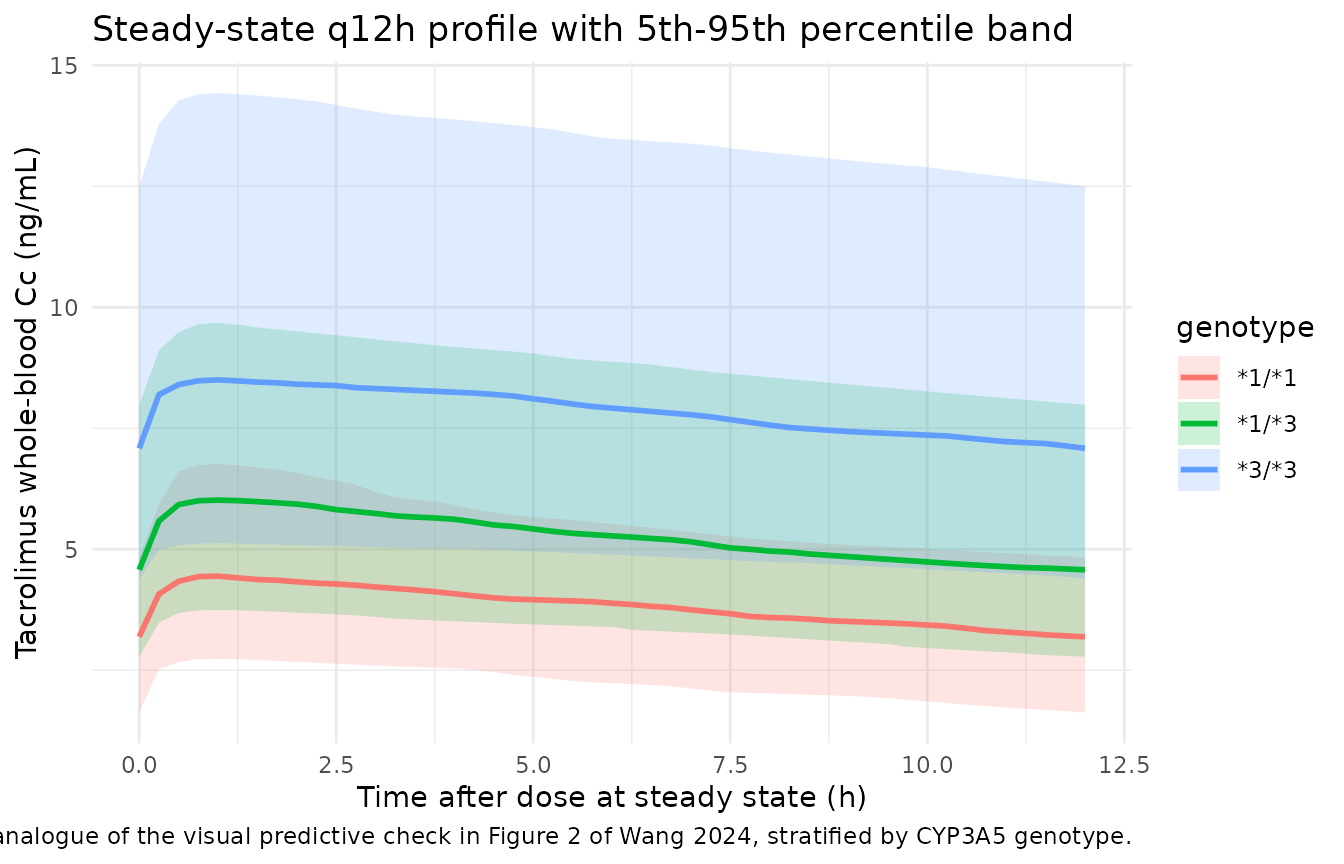
The corresponding typical-value single-dose profiles show the genotype effect on the terminal slope, which is what drives the trough differences above.
sim_sd_typ |>
  dplyr::group_by(genotype, time) |>
  dplyr::summarise(Cc = median(Cc), .groups = "drop") |>
  ggplot(aes(time, Cc, colour = genotype)) +
  geom_line(linewidth = 1) +
  scale_y_log10() +
  labs(
    x = "Time (h)",
    y = "Tacrolimus whole-blood Cc (ng/mL)",
    title = "Typical-value single-dose profiles by CYP3A5 genotype",
    caption = "0.05 mg/kg single oral dose; log scale."
  ) +
  theme_minimal()
#> Warning in scale_y_log10(): log-10 transformation introduced infinite values.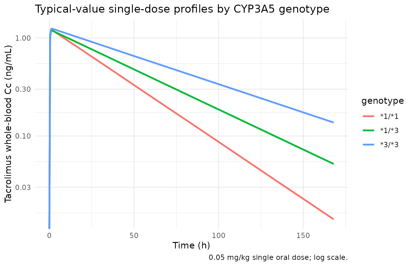
PKNCA validation
Wang 2024 reports no NCA parameters – the dataset contained only pre-dose troughs, so no Cmax, Tmax, AUC, or half-life was ever computed by the authors. There is consequently no published NCA table to compare against. Instead, NCA is run on the simulated single-dose profiles and compared against the exact closed-form values implied by the paper’s own printed parameters (AUC0-inf = Dose / (CL/F) and t1/2 = ln(2) * (V/F) / (CL/F)). This verifies that the packaged encoding reproduces the published equation, which is the verifiable claim available for this paper.
sim_nca <- sim_sd_typ |>
  dplyr::filter(!is.na(Cc)) |>
  dplyr::select(id, time, Cc, genotype)

# Guarantee a time = 0 row per subject; for an extravascular dose the pre-dose
# concentration is 0.
sim_nca <- dplyr::bind_rows(
  sim_nca,
  sim_nca |> dplyr::distinct(id, genotype) |> dplyr::mutate(time = 0, Cc = 0)
) |>
  dplyr::distinct(id, genotype, time, .keep_all = TRUE) |>
  dplyr::arrange(id, genotype, time)

conc_obj <- PKNCA::PKNCAconc(sim_nca, Cc ~ time | genotype + id)

dose_df <- events_sd |>
  dplyr::filter(evid == 1) |>
  dplyr::select(id, time, amt, genotype)

dose_obj <- PKNCA::PKNCAdose(dose_df, amt ~ time | genotype + id)

intervals <- data.frame(
  start      = 0,
  end        = Inf,
  cmax       = TRUE,
  tmax       = TRUE,
  aucinf.obs = TRUE,
  half.life  = TRUE
)

nca_res <- PKNCA::pk.nca(PKNCA::PKNCAdata(conc_obj, dose_obj, intervals = intervals))
Comparison against the closed-form expectation
expected <- analytic |>
  dplyr::group_by(genotype) |>
  dplyr::summarise(
    aucinf.obs = median(aucinf_analytic),
    half.life  = median(halflife_analytic),
    .groups    = "drop"
  )

cmp <- nlmixr2lib::ncaComparisonTable(
  simulated     = nca_res,
  reference     = expected,
  by            = "genotype",
  params        = c("aucinf.obs", "half.life"),
  units         = c(aucinf.obs = "ng*h/mL", half.life = "h"),
  tolerance_pct = 20
)

knitr::kable(
  cmp |> dplyr::mutate(genotype = md_star(genotype)),
  digits  = 2,
  caption = paste(
    "Simulated NCA versus the closed-form values implied by Wang 2024's",
    "printed parameters (AUC0-inf = Dose / (CL/F), t1/2 = ln(2)*(V/F)/(CL/F)).",
    "* marks a difference greater than 20%."
  )
)| NCA parameter | genotype | Reference | Simulated | % diff |
|---|---|---|---|---|
| AUC0-∞ (obs) (ng*h/mL) | *1/*1 | 46.8 | 46.7 | -0.2% |
| AUC0-∞ (obs) (ng*h/mL) | *1/*3 | 64.7 | 64.7 | -0.1% |
| AUC0-∞ (obs) (ng*h/mL) | *3/*3 | 95.5 | 95.4 | -0.1% |
| t½ (h) | *1/*1 | 26.1 | 26.1 | +0.0% |
| t½ (h) | *1/*3 | 36.9 | 36.9 | +0.0% |
| t½ (h) | *3/*3 | 52.2 | 52.2 | +0.0% |
Simulated Cmax and Tmax, for which no closed-form reference is quoted above, are reported for completeness.
as.data.frame(nca_res) |>
  dplyr::filter(PPTESTCD %in% c("cmax", "tmax")) |>
  dplyr::group_by(genotype, PPTESTCD) |>
  dplyr::summarise(median = median(PPORRES), .groups = "drop") |>
  tidyr::pivot_wider(names_from = PPTESTCD, values_from = median) |>
  dplyr::mutate(genotype = md_star(genotype)) |>
  dplyr::rename(
    "CYP3A5 genotype"  = genotype,
    "Cmax (ng/mL)"     = cmax,
    "Tmax (h)"         = tmax
  ) |>
  knitr::kable(
    digits  = 2,
    caption = "Simulated typical-value single-dose Cmax and Tmax by genotype."
)| CYP3A5 genotype | Cmax (ng/mL) | Tmax (h) |
|---|---|---|
| *1/*1 | 1.20 | 1.5 |
| *1/*3 | 1.19 | 1.5 |
| *3/*3 | 1.24 | 1.5 |
The simulated Tmax of about 1.3-1.5 h is somewhat later than the
0.5-1 h peak that Wang 2024’s Introduction quotes for tacrolimus
generally. That is a direct consequence of the fixed absorption rate
constant rather than a translation error: with ka = 3.86
1/h and kel = CL/F / (V/F), the closed-form
tmax = ln(ka/kel) / (ka - kel) is 1.30 h for the
1/1 stratum. Because the model was fitted to pre-dose troughs
only, ka carries no information from these data and the
absorption phase should not be used for inference.
Assumptions and deviations
Absorption rate constant: 3.86 versus 3.84 1/h. Wang 2024 is internally inconsistent about
ka. Table 2 reports3.86 (fixed)in all three model columns (structure model, final model, test-set final model), while Results 3.2 states “The value of ka was fixed at 3.84 h-1”. The packaged model uses the Table 2 value of 3.86 1/h because Table 2 is the paper’s designated parameter table and states it three times. The 0.5% difference is immaterial for a model fitted to pre-dose troughs only, wherekais unidentifiable and was held constant precisely for that reason.Hematocrit is consumed as a volume fraction, not as a percent. The canonical register entry for
HCTininst/references/covariate-columns.mdspecifies percent units, and this model overrides that to L/L, following the same override already made inAndrews_2017_tacrolimus.R. This is not a stylistic choice: Wang 2024 Table 1 reports hematocrit as 0.29 +/- 0.056, and only the fraction reading reconciles the final model with the paper’s own covariate-free structural model (42.1 versus 41.1 L/h; the percent reading gives 1.27 L/h). The reconciliation table above shows the arithmetic. Users supplying a dataset with hematocrit in percent must multiply the column by 0.01.CYP3A5 genotype is encoded as a pair of registered binary indicators. Wang 2024 scores the genotype ordinally (1/1 = 0, 1/3 = 1, 3/3 = 2) and enters that score linearly into a single exponential coefficient. Rather than registering a new CYP3A5 genotype-count covariate – which the register’s
CYP3A5_EXPRentry explicitly discourages – the model reconstructs the score insidemodel()from the existingCYP3A5_STAR1_HETandCYP3A5_STAR1_HOMindicators as2 - (2 * CYP3A5_STAR1_HOM + CYP3A5_STAR1_HET). This is exact for all three strata. Note that the reference orientation differs fromPassey_2011_tacrolimus.R, which uses the same indicator pair but anchors at 3/3; Wang 2024 anchors at 1/1, so the reported 70.6 L/h is the 1/1 clearance.Inter-individual variability is read as a standard deviation in percent, not as a CV%. Wang 2024 Table 2 labels its two IIV rows “omega V/F (%)” and “omega CL/F (%)” – that is, omega itself expressed as a percentage – so the encoded variances are
(percent/100)^2(0.4225 and 0.0529) rather than the log-normal back-transformlog(1 + CV^2)(which would give 0.3525 and 0.0503). The Discussion corroborates the SD reading arithmetically: it reports that adding CYP3A5 genotype produced “an 8.85% decrease in interindividual variation in CL/F”, and 31.8 - 8.85 = 22.95, matching the reported final omega CL/F of 23.0 – a difference of percentage points on the omega scale, not a ratio. The two readings differ negligibly for CL/F and by about 20% in variance for V/F; downstream users who prefer the CV% convention should setetalvc ~ 0.3525andetalcl ~ 0.0503.CL/F is anchored at a non-physiological hematocrit of 0. Wang 2024’s printed equation is uncentred in both covariates, so
lcl = log(70.6)is the clearance at HCT = 0 L/L in a 1/1 patient. The equation is encoded exactly as printed rather than re-centred at the cohort mean, so that the packaged parameter matches Table 2 theta3 verbatim. At the training-set mean hematocrit the 1/1 typical CL/F is 68.1 L/h.Only the population PK layer is packaged. Wang 2024’s MLP, SVR, and XGBoost models (Table 3 hyperparameters, Table 4 performance) consume the PK model’s post hoc individual predictions as one tabular feature among many. They are not ODE models and are outside the scope of
nlmixr2lib. The covariates that the machine-learning layer used but the PK model did not retain – most notably postoperative date, which ranks second in the paper’s SHAP analysis – are documented in the model file’scovariatesDataExcludedmetadata.The final model was fitted to the training split only. Table 2’s “Final model” column (n = 103) is what is encoded. The “Test set final model” column (n = 24; V/F 2330 L, CL/F 114 L/h, HCT -0.161, CYP3A5 -0.395) is a refit used for validation and is not packaged. Wang 2024 also reports the validation group’s size inconsistently – “24 patients, 331 points” in Results 3.2 versus “n = 328” in the Figure 4 caption; neither number is used by this model.
No published NCA table exists for comparison. The dataset was pre-dose troughs only, so the paper reports no Cmax, Tmax, AUC, or half-life. The PKNCA section above therefore compares simulated NCA against the exact closed-form values implied by the paper’s own parameters rather than against transcribed published values.
Virtual-cohort distributions are assumptions. Hematocrit and body weight are drawn as independent truncated normals matching the Table 1 training-set means and standard deviations; Wang 2024 reports no correlation structure or distributional shape. Body weight affects only the simulated dose, not any model parameter.
A supplement is referenced but is not required. Wang 2024 links supplementary material at the publisher. Every parameter, the covariate equation, the genotype scoring, the IIV form, and the residual-error form are all printed in the main text and tables, so no value in this model file depends on the supplement.