Lamotrigine (Wang 2019)
Source:vignettes/articles/Wang_2019_lamotrigine.Rmd
Wang_2019_lamotrigine.RmdModel and source
- Citation: Wang Z-z, Zhang Y-f, Huang W-c, Wang X-p, Ni X-j, Lu H-y, Hu J-q, Deng S-h, Zhu X-q, Xie H-s, Chen H-z, Zhang M, Qiu C, Wen Y-g, Shang D-w. Effects of comedication and genetic factors on the population pharmacokinetics of lamotrigine: a prospective analysis in Chinese patients with epilepsy. Front Pharmacol. 2019;10:832. doi:10.3389/fphar.2019.00832. PMCID PMC6669232. Parameters from Table 4 (final model); cohort demographics from Table 1; genotype frequencies from Tables 2 and 3.
- Description: One-compartment population pharmacokinetic model with first-order absorption and first-order elimination for oral lamotrigine (LTG) in 89 Chinese patients with epilepsy (4-63 years) sampled sparsely at steady-state trough (Wang 2019 Table 4, final model). Ka was FIXED at 1.97 1/h from the literature because sampling carried no absorption-phase information. Apparent oral clearance (CL/F) carries three multiplicative fractional covariate factors: concomitant valproic acid (-38.6%), concomitant rifampicin (+64.7%) and the SLC22A1 1222G>A (rs628031) AA genotype (-52.5%). Apparent volume (V/F) carries two: the ABCG2 34G>A (rs2231137) AA genotype (-42.0%) and the combined MDR1/ABCB1 2677TT + 3435TT genotype pair (+139%). Interindividual variability is exponential on CL/F and V/F; residual error is combined additive plus proportional.
- Article (open access): https://doi.org/10.3389/fphar.2019.00832
- PubMed Central: https://www.ncbi.nlm.nih.gov/pmc/articles/PMC6669232/
mod <- rxode2::rxode(readModelDb("Wang_2019_lamotrigine"))
#> ℹ parameter labels from comments will be replaced by 'label()'

# The model defines `cl` and `vc` alongside explicit `d/dt()` states. rxode2
# will silently replace the ODEs with its analytic solution if the pair is
# interpreted as a `linCmt()` request, so confirm that has NOT happened -- every
# check below is meant to exercise the written ODEs.
stopifnot(is.null(mod$linCmt))
Population
Eighty-nine out-patients with epilepsy (42 male, 47 female) contributed 419 lamotrigine serum concentrations in a prospective therapeutic-drug-monitoring study run between July 2014 and January 2017 at Guangzhou Huiai Hospital, the Affiliated Brain Hospital of Guangzhou Medical University, China (Table 1). Mean age was 28 years (range 4-63) and mean body weight 59 kg (range 15-94). The mean lamotrigine dose was 118 mg (range 6.25-300 mg) and the mean duration of therapy 42.8 weeks (range 4-204).
Comedication status was recorded at each sampling time point rather than once per subject, so the two comedication covariates are genuinely time-varying within a patient: 187 observations (44.6%) were on lamotrigine alone, 157 (37.5%) on lamotrigine plus valproic acid, 57 (13.6%) on lamotrigine plus rifampicin, and 19 (4.5%) on both.
Samples were drawn sparsely at steady state, after at least 7 days on
the same dose, and “mainly at 0.5 and 1 h prior to the next dosing”
(Methods). The dataset is therefore essentially trough-only and carries
no absorption-phase information – which is why Ka is FIXED
rather than estimated. Serum lamotrigine was quantified by HPLC-MS/MS
over 0.20-25.00 ug/mL with an LLOQ of 0.20 ug/mL.
The final model was evaluated by NPDE (mean 0.0106, variance 0.953, p = 0.504) and externally validated against an independent retrospective TDM cohort of 114 patients with 384 concentrations (mean prediction error 2.8 mg/L, RMSE 4.8 mg/L). The authors restrict the model’s recommended applicability to patients 13-65 years of age because very young children were under-represented (Discussion).
The same information is available programmatically via
readModelDb("Wang_2019_lamotrigine")()$population.
Source trace
Every ini() entry in
inst/modeldb/specificDrugs/Wang_2019_lamotrigine.R carries
an in-file comment naming its origin. They are collected here for
review.
| Equation / parameter | Value | Source location |
|---|---|---|
lka (Ka) |
1.97 1/h, FIXED | Methods, “Population Pharmacokinetic Modeling”; Table 4 row
K a, 1/h prints 1.97 FIX
|
lcl (CL/F) |
1.12 L/h | Table 4, final model (%CV 14.6; bootstrap 95% CI 0.95-1.52) |
lvc (V/F) |
12.7 L | Table 4, final model (%CV 28.4; bootstrap 95% CI 9.57-20.38) |
e_conmed_vpa_cl |
-0.386 | Table 4 row theta VPA on CL/F (%CV 19.1; CI -0.55 to
-0.25) |
e_conmed_rif_cl |
0.647 | Table 4 row theta RFP on CL/F (%CV 15.4; CI
0.48-0.86) |
e_snp_slc22a1_rs628031_hom_cl |
-0.525 | Table 4 row theta SLC22A1-1222 AA on CL/F (%CV 29.5; CI
-0.79 to -0.19) |
e_snp_abcg2_rs2231137_hom_vc |
-0.420 | Table 4 row theta ABCG2-34 AA on V/F (%CV 35.5; CI
-0.65 to -0.14) |
e_snp_abcb1_2677tt_3435tt_vc |
1.390 | Table 4 row theta MDR1-2677 TT + C3435 TT on V/F (%CV
43.0; CI 0.21-3.25) |
etalcl |
0.02284 = log(1 + 0.152^2) | Table 4 row CL INTER VAR, % final = 15.2 |
etalvc |
0.03961 = log(1 + 0.201^2) | Table 4 row V INTER VAR, % final = 20.1 |
addSd |
0.797 mg/L | Table 4 row Additive error, mg/L final (%CV 31.0; CI
0.28-1.35) |
propSd |
0.167 | Table 4 row Proportional error, % final (%CV 24.4; CI
10.24-20.77%) |
Fractional covariate form
P = Ptv * (1 + theta * COV)
|
n/a | Methods, “Population Pharmacokinetic Modeling” |
| Multiplicative combination across covariates | n/a | Results, final-model E factors (“otherwise
corresponding E value was assigned 1”) |
| Combined MDR1 2677TT + 3435TT covariate | n/a | Results paragraph 2 and Discussion (“91.67%” co-occurrence) |
| One compartment, first-order in and out | n/a | Methods and Results, “Population Pharmacokinetic Modeling” |
Virtual cohort
Original observed data are not publicly available. Wang 2019’s own validation figures are simulations rather than observed-data overlays: Figure 4A shows steady-state profiles for six patient types at a common 100 mg twice-daily dose and Figure 4B shows the same six types at personalised doses. Both are reproduced below.
The six patient types are exactly those the paper enumerates (Methods, “Simulations to Achieve Target Concentrations”), plus a seventh – concurrent valproic acid and rifampicin – used to test the paper’s “offset” claim in the Discussion.
tau <- 12 # 100 mg b.i.d.

patient_types <- tibble::tibble(
  type = factor(
    c(
      "Ordinary", "VPA", "RFP", "SLC22A1-1222AA", "ABCG2-34AA",
      "MDR1-2677TT+3435TT", "VPA + RFP"
    ),
    levels = c(
      "Ordinary", "VPA", "RFP", "SLC22A1-1222AA", "ABCG2-34AA",
      "MDR1-2677TT+3435TT", "VPA + RFP"
    )
  ),
  CONMED_VPA = c(0, 1, 0, 0, 0, 0, 1),
  CONMED_RIF = c(0, 0, 1, 0, 0, 0, 1),
  SNP_SLC22A1_RS628031_HOM = c(0, 0, 0, 1, 0, 0, 0),
  SNP_ABCG2_RS2231137_HOM = c(0, 0, 0, 0, 1, 0, 0),
  SNP_ABCB1_RS2032582_HOM = c(0, 0, 0, 0, 0, 1, 0),
  SNP_ABCB1_RS1045642_HOM = c(0, 0, 0, 0, 0, 1, 0)
) |>
  dplyr::mutate(id = dplyr::row_number())

knitr::kable(patient_types, caption = "The six Wang 2019 patient types plus the VPA + RFP combination.")| type | CONMED_VPA | CONMED_RIF | SNP_SLC22A1_RS628031_HOM | SNP_ABCG2_RS2231137_HOM | SNP_ABCB1_RS2032582_HOM | SNP_ABCB1_RS1045642_HOM | id |
|---|---|---|---|---|---|---|---|
| Ordinary | 0 | 0 | 0 | 0 | 0 | 0 | 1 |
| VPA | 1 | 0 | 0 | 0 | 0 | 0 | 2 |
| RFP | 0 | 1 | 0 | 0 | 0 | 0 | 3 |
| SLC22A1-1222AA | 0 | 0 | 1 | 0 | 0 | 0 | 4 |
| ABCG2-34AA | 0 | 0 | 0 | 1 | 0 | 0 | 5 |
| MDR1-2677TT+3435TT | 0 | 0 | 0 | 0 | 1 | 1 | 6 |
| VPA + RFP | 1 | 1 | 0 | 0 | 0 | 0 | 7 |
Covariate factors reproduce the published effect sizes
Before simulating anything, the encoded coefficients are checked directly against the percentages the paper states in its Abstract and Results.
th <- mod$theta

cov_check <- tibble::tibble(
  Covariate = c(
    "VPA on CL/F", "RFP on CL/F", "SLC22A1-1222AA on CL/F",
    "ABCG2-34AA on V/F", "MDR1-2677TT+3435TT on V/F"
  ),
  coefficient = c(
    th[["e_conmed_vpa_cl"]], th[["e_conmed_rif_cl"]],
    th[["e_snp_slc22a1_rs628031_hom_cl"]],
    th[["e_snp_abcg2_rs2231137_hom_vc"]],
    th[["e_snp_abcb1_2677tt_3435tt_vc"]]
  ),
  factor = 1 + coefficient,
  published_pct_change = c(-38.5, 64.7, -52.5, -42.0, 136)
) |>
  dplyr::mutate(encoded_pct_change = 100 * coefficient)

cov_check |>
  dplyr::rename(
    "Coefficient (theta)" = coefficient,
    "Factor E = 1 + theta" = factor,
    "Published % change" = published_pct_change,
    "Encoded % change" = encoded_pct_change
  ) |>
knitr::kable(digits = 3, caption = "Encoded covariate coefficients vs the percentages stated in Wang 2019.")| Covariate | Coefficient (theta) | Factor E = 1 + theta | Published % change | Encoded % change |
|---|---|---|---|---|
| VPA on CL/F | -0.386 | 0.614 | -38.5 | -38.6 |
| RFP on CL/F | 0.647 | 1.647 | 64.7 | 64.7 |
| SLC22A1-1222AA on CL/F | -0.525 | 0.475 | -52.5 | -52.5 |
| ABCG2-34AA on V/F | -0.420 | 0.580 | -42.0 | -42.0 |
| MDR1-2677TT+3435TT on V/F | 1.390 | 2.390 | 136.0 | 139.0 |
# Each encoded effect must land within half a percentage point of the published
# figure. The MDR1 row is the one the paper itself states two ways -- 136% /
# 2.36-fold in prose, 1.390 / 2.390-fold in Table 4 and in the E-factor list --
# so it gets the wider tolerance the paper's own disagreement forces.
stopifnot(
  all(abs(cov_check$encoded_pct_change[1:4] - cov_check$published_pct_change[1:4]) < 0.6),
  abs(cov_check$encoded_pct_change[5] - cov_check$published_pct_change[5]) < 4
)

# Discussion: "when VPA and RFP were administered together with LTG, the effect
# on the CL/F of LTG was offset." That is only true of a MULTIPLICATIVE
# combination -- it is the arithmetic that fixes the covariate model's form.
offset_factor <- (1 + th[["e_conmed_vpa_cl"]]) * (1 + th[["e_conmed_rif_cl"]])
offset_factor
#> [1] 1.011258
stopifnot(abs(offset_factor - 1) < 0.02)
Steady-state simulation: replicating Figure 4A
Wang 2019 simulated “concentrations of 0, 0.5, and 1 h prior to the next dosing from the first dose to the steady state on the basis of a commonly used dose of 100 mg twice daily (b.i.d.)” for the six patient types, and evaluated the result against an assumed optimum range of 3-5 ug/mL.
Typical-value profiles are used for the published-claim checks
(rxode2::zeroRe() removes the random effects), so the
assertions below depend only on the encoded parameter values and not on
any draw.
build_events <- function(types, dose_mg, tau, n_days = 21) {
  dosing <- tidyr::expand_grid(
    types,
    tibble::tibble(time = seq(0, (n_days - 1) * 24, by = tau))
  ) |>
    dplyr::mutate(evid = 1L, amt = dose_mg, cmt = "depot", dv = NA_real_)

  # Observations are placed on the ODE state `central`; rxode2 returns the
  # algebraic observable as a column at those rows. Never name an algebraic
  # observable in the compartment column -- that injects a compartment slot
  # after the ODE states and renumbers every one of them.
  obs <- tidyr::expand_grid(
    types,
    tibble::tibble(time = seq(0, n_days * 24, by = 0.25))
  ) |>
    dplyr::mutate(evid = 0L, amt = NA_real_, cmt = "central", dv = NA_real_)

  dplyr::bind_rows(dosing, obs) |>
    dplyr::arrange(id, time, dplyr::desc(evid)) |>
    as.data.frame()
}

# `dose_mg` is length-1 here; when it varies per arm it must be joined onto the
# type table rather than recycled positionally.
ev_100 <- build_events(patient_types, dose_mg = 100, tau = tau)

mod_typ <- rxode2::zeroRe(mod)
sim_100 <- rxode2::rxSolve(
  mod_typ,
  ev_100,
  keep = c("type"),
  returnType = "data.frame"
)
#> ℹ omega/sigma items treated as zero: 'etalcl', 'etalvc'
#> Warning: multi-subject simulation without without 'omega'
ss_start <- 20 * 24 # the 41st dose; >= 10 half-lives for every patient type

sim_100 |>
  dplyr::filter(time >= ss_start, time <= ss_start + tau) |>
  dplyr::mutate(time_in_interval = time - ss_start) |>
  ggplot2::ggplot(ggplot2::aes(time_in_interval, Cc, colour = type)) +
  ggplot2::annotate("rect", xmin = -Inf, xmax = Inf, ymin = 3, ymax = 5, alpha = 0.12) +
  ggplot2::geom_line(linewidth = 0.8) +
  ggplot2::labs(
    x = "Time within the steady-state dosing interval (h)",
    y = "Lamotrigine concentration (mg/L)",
    colour = "Patient type"
  ) +
  ggplot2::theme_bw()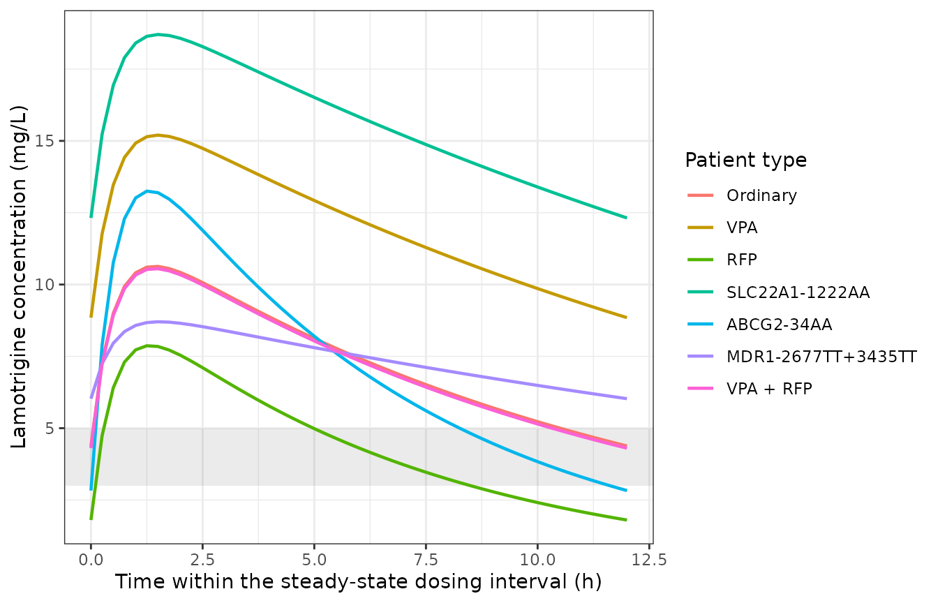
Replicates Figure 4A of Wang 2019: typical-value steady-state lamotrigine profiles at 100 mg b.i.d. for six patient types. The shaded band is the 3-5 ug/mL optimum range assumed by the authors.
The published Figure 4A claims, as assertions
The trough and the 1-h-pre-dose concentration are extracted for each patient type, because those are the sampling times the paper simulated.
ss <- sim_100 |>
  dplyr::filter(time >= ss_start, time <= ss_start + tau) |>
  dplyr::mutate(time_in_interval = round(time - ss_start, 6))

ss_summary <- ss |>
  dplyr::group_by(type) |>
  dplyr::summarise(
    cmax = max(Cc),
    ctrough = Cc[time_in_interval == tau],
    c_1h_predose = Cc[time_in_interval == tau - 1],
    .groups = "drop"
  )

ss_summary |>
  dplyr::rename(
    "Patient type" = type,
    "Cmax,ss (mg/L)" = cmax,
    "Ctrough,ss (mg/L)" = ctrough,
    "C 1 h pre-dose (mg/L)" = c_1h_predose
  ) |>
knitr::kable(digits = 2, caption = "Steady-state exposure at 100 mg b.i.d. by patient type.")| Patient type | Cmax,ss (mg/L) | Ctrough,ss (mg/L) | C 1 h pre-dose (mg/L) |
|---|---|---|---|
| Ordinary | 10.63 | 4.38 | 4.79 |
| VPA | 15.20 | 8.85 | 9.34 |
| RFP | 7.87 | 1.80 | 2.09 |
| SLC22A1-1222AA | 18.70 | 12.32 | 12.84 |
| ABCG2-34AA | 13.25 | 2.83 | 3.29 |
| MDR1-2677TT+3435TT | 8.70 | 6.03 | 6.25 |
| VPA + RFP | 10.55 | 4.30 | 4.71 |
get_ss <- function(what, which_type) {
  ss_summary[[what]][ss_summary$type == which_type]
}

# Claim 1 (Results, "Model Simulation"): "only two types of patients were
# predicted to achieve the target steady-state concentration range (3-5 ug/ml):
# one with the ABCG2-34AA genotype and the other with no gene mutation or
# comedication with VPA or RFP, for which dosage adjustment might not be
# necessary." The paper sampled 0, 0.5 and 1 h pre-dose, so the ABCG2 arm is
# judged on that window rather than on the 12-h trough alone.
stopifnot(
  get_ss("ctrough", "Ordinary") > 3, get_ss("ctrough", "Ordinary") < 5,
  get_ss("c_1h_predose", "Ordinary") > 3, get_ss("c_1h_predose", "Ordinary") < 5,
  get_ss("c_1h_predose", "ABCG2-34AA") > 3, get_ss("c_1h_predose", "ABCG2-34AA") < 5
)

# Claim 2: "the comedication with RFP induced an obvious decrease in LTG
# exposure, which resulted in underexposure of LTG below the target level".
stopifnot(get_ss("c_1h_predose", "RFP") < 3)

# Claim 3: "comedication with VPA or the genotype SLC22A1-1222AA resulted in a
# large increase in LTG exposure up to ~13 ug/ml, more than two-fold above the
# upper target level". The stated ceiling is the larger of the two arms.
stopifnot(
  get_ss("ctrough", "SLC22A1-1222AA") > 11,
  get_ss("ctrough", "SLC22A1-1222AA") < 14,
  get_ss("ctrough", "VPA") > 5,
  get_ss("ctrough", "VPA") < get_ss("ctrough", "SLC22A1-1222AA")
)

# Claim 4: "MDR1 TT carriers showed a slight increase in steady-state
# concentration" -- above the ordinary patient, but far below the VPA and
# SLC22A1 arms.
stopifnot(
  get_ss("ctrough", "MDR1-2677TT+3435TT") > get_ss("ctrough", "Ordinary"),
  get_ss("ctrough", "MDR1-2677TT+3435TT") < get_ss("ctrough", "VPA")
)

# Claim 5 (Discussion): concurrent VPA and RFP offset one another, so that arm
# must sit within a couple of percent of the ordinary patient.
stopifnot(
  abs(get_ss("ctrough", "VPA + RFP") / get_ss("ctrough", "Ordinary") - 1) < 0.03
)
PKNCA validation
Non-compartmental analysis is run over the steady-state dosing interval with PKNCA, and compared against the closed-form one-compartment oral solution evaluated at the same encoded parameter values. This is a self-consistency gate on the ODE encoding – Wang 2019 publishes no NCA table, so there is no external NCA reference to compare to; the external comparison is the Figure 4A and 4B reproduction above and below.
conc_df <- sim_100 |>
  dplyr::filter(!is.na(Cc)) |>
  dplyr::select(id, type, time, Cc)

# `ev_100` already carries `type` (build_events() expands the patient-type
# table), so joining it back on would create type.x / type.y.
dose_df <- ev_100 |>
  dplyr::filter(evid == 1) |>
  dplyr::select(id, type, time, amt)

conc_obj <- PKNCA::PKNCAconc(
  data = as.data.frame(conc_df),
  formula = Cc ~ time | type + id,
  concu = "mg/L",
  timeu = "h"
)
dose_obj <- PKNCA::PKNCAdose(
  data = as.data.frame(dose_df),
  formula = amt ~ time | type + id,
  doseu = "mg"
)

intervals <- data.frame(
  start = ss_start,
  end = ss_start + tau,
  cmax = TRUE,
  tmax = TRUE,
  cmin = TRUE,
  auclast = TRUE,
  cav = TRUE,
  half.life = TRUE
)

nca_res <- PKNCA::pk.nca(
  PKNCA::PKNCAdata(conc_obj, dose_obj, intervals = intervals)
)

nca_tbl <- as.data.frame(nca_res$result) |>
  dplyr::filter(PPTESTCD %in% c("cmax", "cmin", "auclast", "cav", "half.life")) |>
  dplyr::select(type, PPTESTCD, PPORRES) |>
  tidyr::pivot_wider(names_from = PPTESTCD, values_from = PPORRES)
# Closed-form reference: one compartment, first-order absorption, at steady
# state with dosing interval tau.
#   C(t) = D*ka/(V*(ka-kel)) * [ exp(-kel t)/(1-exp(-kel tau))
#                              - exp(-ka  t)/(1-exp(-ka  tau)) ]
ka_ref <- exp(th[["lka"]])

analytic <- patient_types |>
  dplyr::mutate(
    cl = exp(th[["lcl"]]) *
      (1 + th[["e_conmed_vpa_cl"]] * CONMED_VPA) *
      (1 + th[["e_conmed_rif_cl"]] * CONMED_RIF) *
      (1 + th[["e_snp_slc22a1_rs628031_hom_cl"]] * SNP_SLC22A1_RS628031_HOM),
    vc = exp(th[["lvc"]]) *
      (1 + th[["e_snp_abcg2_rs2231137_hom_vc"]] * SNP_ABCG2_RS2231137_HOM) *
      (1 + th[["e_snp_abcb1_2677tt_3435tt_vc"]] *
        SNP_ABCB1_RS2032582_HOM * SNP_ABCB1_RS1045642_HOM),
    kel = cl / vc,
    cmin = 100 * ka_ref / (vc * (ka_ref - kel)) *
      (exp(-kel * tau) / (1 - exp(-kel * tau)) -
        exp(-ka_ref * tau) / (1 - exp(-ka_ref * tau))),
    cav = 100 / (cl * tau),
    auclast = 100 / cl,
    half.life = log(2) / kel
  ) |>
  dplyr::select(type, cmin, cav, auclast, half.life)

cmp <- nlmixr2lib::ncaComparisonTable(
  simulated = nca_tbl |> dplyr::select(type, cmin, cav, auclast, half.life),
  reference = analytic,
  by = "type",
  tolerance_pct = 20,
  label_first_column = "NCA parameter"
)
knitr::kable(
  cmp,
  caption = "Steady-state PKNCA output vs the closed-form one-compartment oral solution, by patient type."
)| NCA parameter | type | Reference | Simulated | % diff |
|---|---|---|---|---|
| Cmin | Ordinary | 4.38 | 4.38 | +0.0% |
| Cmin | VPA | 8.85 | 8.85 | -0.0% |
| Cmin | RFP | 1.8 | 1.8 | +0.0% |
| Cmin | SLC22A1-1222AA | 12.3 | 12.3 | -0.0% |
| Cmin | ABCG2-34AA | 2.83 | 2.83 | +0.0% |
| Cmin | MDR1-2677TT+3435TT | 6.03 | 6.03 | -0.0% |
| Cmin | VPA + RFP | 4.3 | 4.3 | +0.0% |
| AUClast | Ordinary | 89.3 | 89.2 | -0.1% |
| AUClast | VPA | 145 | 145 | -0.1% |
| AUClast | RFP | 54.2 | 54.1 | -0.2% |
| AUClast | SLC22A1-1222AA | 188 | 188 | -0.0% |
| AUClast | ABCG2-34AA | 89.3 | 89.1 | -0.2% |
| AUClast | MDR1-2677TT+3435TT | 89.3 | 89.3 | -0.0% |
| AUClast | VPA + RFP | 88.3 | 88.2 | -0.1% |
| t½ | Ordinary | 7.86 | 7.91 | +0.6% |
| t½ | VPA | 12.8 | 12.9 | +0.4% |
| t½ | RFP | 4.77 | 4.8 | +0.5% |
| t½ | SLC22A1-1222AA | 16.5 | 16.6 | +0.4% |
| t½ | ABCG2-34AA | 4.56 | 4.58 | +0.5% |
| t½ | MDR1-2677TT+3435TT | 18.8 | 18.9 | +0.4% |
| t½ | VPA + RFP | 7.77 | 7.82 | +0.6% |
| Cavg | Ordinary | 7.44 | 7.43 | -0.1% |
| Cavg | VPA | 12.1 | 12.1 | -0.1% |
| Cavg | RFP | 4.52 | 4.51 | -0.2% |
| Cavg | SLC22A1-1222AA | 15.7 | 15.7 | -0.0% |
| Cavg | ABCG2-34AA | 7.44 | 7.43 | -0.2% |
| Cavg | MDR1-2677TT+3435TT | 7.44 | 7.44 | -0.0% |
| Cavg | VPA + RFP | 7.36 | 7.35 | -0.1% |
gate <- nca_tbl |>
  dplyr::select(type, cmin, cav, auclast, half.life) |>
  dplyr::left_join(analytic, by = "type", suffix = c("_sim", "_ref"))

# Both sides use the SAME parameters -- the only differences are ODE
# integration, trapezoidal quadrature on a 0.25 h grid, and (for half-life)
# log-linear regression -- so tight all()-bounds are correct here and must be
# kept. These are numerical-error bounds, not cohort extremes.
#
# Cmin is read off the grid directly and matches to 1e-4. AUC and Cav carry
# trapezoidal error and match to 1e-3. Half-life is the loosest of the three at
# 1e-2, because PKNCA's lambda-z regression runs over a 12 h steady-state
# interval that still carries a trace of the absorption phase (Ka = 1.97 1/h);
# the observed bias is a consistent +0.4 to +0.6% on every arm.
stopifnot(
  max(abs(gate$cmin_sim / gate$cmin_ref - 1)) < 1e-4,
  max(abs(gate$cav_sim / gate$cav_ref - 1)) < 2e-3,
  max(abs(gate$half.life_sim / gate$half.life_ref - 1)) < 1e-2
)

# Dose recovery at steady state: because CL/F and V/F are APPARENT parameters,
# F is folded into them and the identity is CL/F * AUC(0-tau),ss = Dose exactly.
# This is the gate that would catch a mis-encoded absorption path or a lost
# dose, which the Cmin check alone cannot.
stopifnot(max(abs(gate$auclast_sim / gate$auclast_ref - 1)) < 2e-3)

# Mutation control: the recovery gate must FAIL when the dose is wrong, proving
# it is not vacuous.
stopifnot(any(abs((gate$auclast_sim * 2) / gate$auclast_ref - 1) > 2e-3))
Personalised dose regimens: replicating Figure 4B
Wang 2019’s second simulation scenario adjusts the dose per patient type to land inside the 3-5 ug/mL window, and the Results and Discussion state three of the adjusted doses explicitly:
- SLC22A1-1222AA carriers: “given a dose (37.5 mg b.i.d.) approximately one-third the normal dosage”;
- rifampicin comedication: “a 125% increase in dose was suggested”, i.e. 225 mg b.i.d. (“Coadministration with RFP caused the dose to increase 2.25-fold over the normal dosage”);
- valproate comedication: “the LTG dose should be decreased by 50% when the therapy is combined with VPA …, in agreement with our simulated results in Figure 4”, i.e. 50 mg b.i.d.
Each is simulated below and required to land inside the target window. These are genuine external checks: the doses are published numbers that the encoded model was not fitted to.
personalised <- tibble::tribble(
  ~type, ~dose_mg,
  "Ordinary", 100,
  "VPA", 50,
  "RFP", 225,
  "SLC22A1-1222AA", 37.5,
  "ABCG2-34AA", 100
)

sim_personalised <- lapply(seq_len(nrow(personalised)), function(i) {
  ty <- patient_types |> dplyr::filter(type == personalised$type[i])
  ev <- build_events(ty, dose_mg = personalised$dose_mg[i], tau = tau)
  out <- rxode2::rxSolve(mod_typ, ev, keep = c("type"), returnType = "data.frame")
  out$dose_mg <- personalised$dose_mg[i]
  out
}) |>
  dplyr::bind_rows()
#> ℹ omega/sigma items treated as zero: 'etalcl', 'etalvc'
#> ℹ omega/sigma items treated as zero: 'etalcl', 'etalvc'
#> ℹ omega/sigma items treated as zero: 'etalcl', 'etalvc'
#> ℹ omega/sigma items treated as zero: 'etalcl', 'etalvc'
#> ℹ omega/sigma items treated as zero: 'etalcl', 'etalvc'

personalised_ss <- sim_personalised |>
  dplyr::filter(time >= ss_start, time <= ss_start + tau) |>
  dplyr::mutate(time_in_interval = round(time - ss_start, 6)) |>
  dplyr::group_by(type, dose_mg) |>
  dplyr::summarise(
    ctrough = Cc[time_in_interval == tau],
    c_1h_predose = Cc[time_in_interval == tau - 1],
    .groups = "drop"
  )

personalised_ss |>
  dplyr::rename(
    "Patient type" = type,
    "Dose (mg b.i.d.)" = dose_mg,
    "Ctrough,ss (mg/L)" = ctrough,
    "C 1 h pre-dose (mg/L)" = c_1h_predose
  ) |>
knitr::kable(digits = 2, caption = "Replicates Figure 4B of Wang 2019: personalised doses and the resulting steady-state exposure.")| Patient type | Dose (mg b.i.d.) | Ctrough,ss (mg/L) | C 1 h pre-dose (mg/L) |
|---|---|---|---|
| Ordinary | 100.0 | 4.38 | 4.79 |
| VPA | 50.0 | 4.42 | 4.67 |
| RFP | 225.0 | 4.06 | 4.69 |
| SLC22A1-1222AA | 37.5 | 4.62 | 4.82 |
| ABCG2-34AA | 100.0 | 2.83 | 3.29 |
# Every published personalised dose must put the pre-dose window inside 3-5
# ug/mL. The paper's stated recommended range is 37.5-225 mg b.i.d.
stopifnot(
  all(personalised_ss$c_1h_predose > 3),
  all(personalised_ss$c_1h_predose < 5.5),
  min(personalised$dose_mg) == 37.5,
  max(personalised$dose_mg) == 225
)
sim_personalised |>
  dplyr::filter(time >= ss_start, time <= ss_start + tau) |>
  dplyr::mutate(
    time_in_interval = time - ss_start,
    arm = paste0(type, " (", dose_mg, " mg)")
  ) |>
  ggplot2::ggplot(ggplot2::aes(time_in_interval, Cc, colour = arm)) +
  ggplot2::annotate("rect", xmin = -Inf, xmax = Inf, ymin = 3, ymax = 5, alpha = 0.12) +
  ggplot2::geom_line(linewidth = 0.8) +
  ggplot2::labs(
    x = "Time within the steady-state dosing interval (h)",
    y = "Lamotrigine concentration (mg/L)",
    colour = "Arm (dose)"
  ) +
  ggplot2::theme_bw()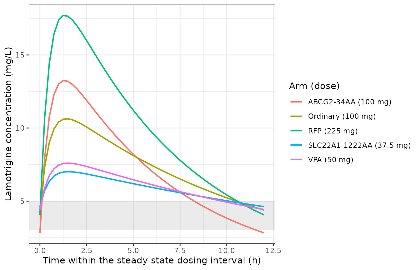
Replicates Figure 4B of Wang 2019: steady-state profiles at the published personalised doses. The shaded band is the 3-5 ug/mL target.
Time to steady state
The paper states that “the target steady-state concentration was achieved after continuous dosing for at least 3 days” and that “more rapid achievement of the target steady-state concentration was observed in the normal, ABCG2, and RFP groups within 2 days” (Results, “Model Simulation”). Both follow from the elimination half-lives the encoded parameters imply.
thalf <- analytic |>
  dplyr::select(type, half.life) |>
  dplyr::mutate(days_to_90pct_ss = half.life * log(10) / log(2) / 24)

thalf |>
  dplyr::rename(
    "Patient type" = type,
    "t1/2 (h)" = half.life,
    "Days to 90% of steady state" = days_to_90pct_ss
  ) |>
knitr::kable(digits = 2, caption = "Elimination half-life and time to 90% of steady state by patient type.")| Patient type | t1/2 (h) | Days to 90% of steady state |
|---|---|---|
| Ordinary | 7.86 | 1.09 |
| VPA | 12.80 | 1.77 |
| RFP | 4.77 | 0.66 |
| SLC22A1-1222AA | 16.55 | 2.29 |
| ABCG2-34AA | 4.56 | 0.63 |
| MDR1-2677TT+3435TT | 18.78 | 2.60 |
| VPA + RFP | 7.77 | 1.08 |
Stochastic cohort
A modest virtual cohort illustrates the interindividual variability
the model carries (etalcl 15.2% CV, etalvc
20.1% CV). No assertion is made on this cohort:
rxode2::rxSetSeed() fixes the draw within an rxode2 version
and thread count but not across them, so an assertion on a simulated
extreme is not reproducible in CI.
rxode2::rxSetSeed(20190725)

n_per_arm <- 100 # cap is 200 per arm

vpc_types <- patient_types |>
  dplyr::filter(type %in% c("Ordinary", "VPA")) |>
  dplyr::select(-id) |>
  dplyr::slice(rep(seq_len(2), each = n_per_arm)) |>
  dplyr::mutate(id = dplyr::row_number())

ev_vpc <- build_events(vpc_types, dose_mg = 100, tau = tau, n_days = 21) |>
  dplyr::filter(evid == 1 | time >= ss_start)

sim_vpc <- rxode2::rxSolve(mod, ev_vpc, keep = c("type"), returnType = "data.frame")

sim_vpc |>
  dplyr::filter(time >= ss_start, time <= ss_start + tau) |>
  dplyr::mutate(time_in_interval = time - ss_start) |>
  dplyr::group_by(type, time_in_interval) |>
  dplyr::summarise(
    lo = quantile(Cc, 0.05),
    mid = median(Cc),
    hi = quantile(Cc, 0.95),
    .groups = "drop"
  ) |>
  ggplot2::ggplot(ggplot2::aes(time_in_interval, mid, fill = type, colour = type)) +
  ggplot2::annotate("rect", xmin = -Inf, xmax = Inf, ymin = 3, ymax = 5, alpha = 0.12) +
  ggplot2::geom_ribbon(ggplot2::aes(ymin = lo, ymax = hi), alpha = 0.25, colour = NA) +
  ggplot2::geom_line(linewidth = 0.8) +
  ggplot2::labs(
    x = "Time within the steady-state dosing interval (h)",
    y = "Lamotrigine concentration (mg/L)",
    fill = "Patient type", colour = "Patient type"
  ) +
  ggplot2::theme_bw()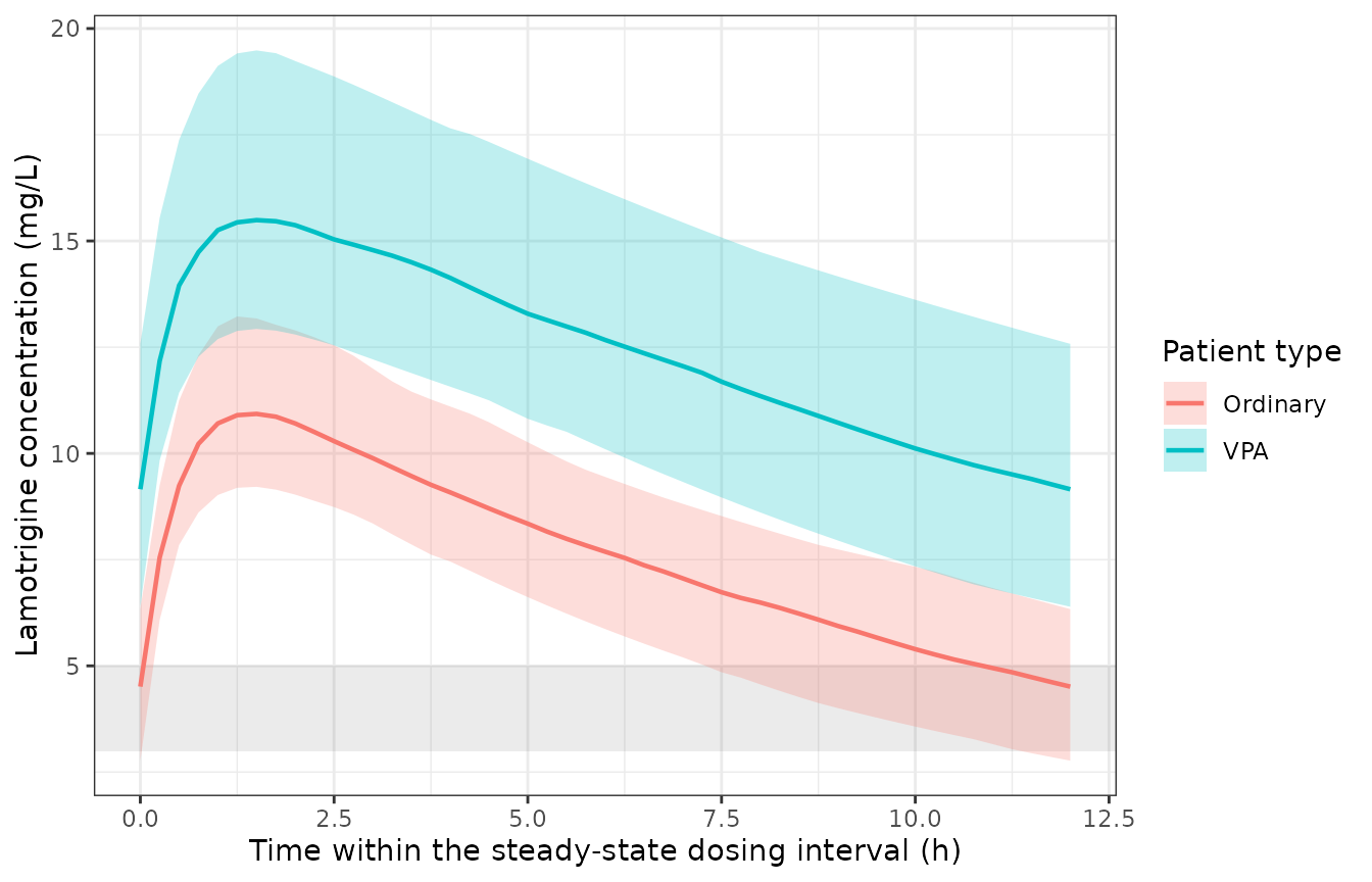
Steady-state variability at 100 mg b.i.d. for the ordinary and VPA-comedicated patient types (100 subjects per arm, typical-value profile overlaid in black).
Assumptions and deviations
Errata and internal inconsistencies in Wang 2019
The Results paragraph’s restated
Efactors disagree with Table 4 for two of five covariates. The paper writes the final model as multiplicative factors with values 0.624 (VPA), 1.647 (RFP), 0.475 (SLC22A1-1222AA), 0.680 (ABCG2-34AA) and 2.390 (MDR1-2677TT+3435TT). Table 4’sthetacolumn gives -0.386, 0.647, -0.525, -0.420 and 1.390, which imply factors of 0.614, 1.647, 0.475, 0.580 and 2.390. Three of five agree exactly; VPA and ABCG2 do not. The Table 4 values are used, for three independent reasons: (a) Table 4 is the fitted-parameter table and is the only place the %CV and bootstrap confidence intervals are printed; (b) the Abstract and the Results narrative both state the ABCG2 effect as a “42.0% decrease in V/F”, which is 0.580 and not 0.680, and both state the VPA effect as a “38.5% decrease”, which is 0.615 and not 0.624; (c) the Discussion’s claim that concurrent VPA and RFP “offset” one another holds for 0.614 x 1.647 = 1.011 and less well for 0.624 x 1.647 = 1.028. TheEvalues look like single-digit typesetting slips.The MDR1 effect is stated two ways. Table 4 and the
Elist agree on 1.390 / 2.390-fold, while the Abstract and Results prose say “136% (2.36-fold) increase”. Table 4 is used, as above; the covariate-factor assertion widens its tolerance for this row alone to accommodate the paper’s own disagreement.The fixed
Kais attributed to two different references. The Methods and the Discussion limitations both cite Milosheska 2016 for the fixed 1.97 1/h; the Results paragraph cites Liu 2015 instead. Milosheska 2016 is the lamotrigine PK paper of the two and is also packaged here (Milosheska_2016_lamotrigine), where the estimatedKais 1.96 1/h (95% CI 1.72-2.24) – so Wang 2019’s 1.97 is a rounding of the Milosheska value, confirming that attribution. Liu 2015 is a study of valproate concentration and UGT polymorphism in children and reports noKa. The model uses Wang 2019’s printed 1.97, which is the value they actually fixed.The proportional residual error is printed in a
%-labelled row as a fraction. Table 4’sProportional error, %row gives 21.8 for the base model (a percent) but 0.167 for the final model (a fraction), with a bootstrap CI of 10.24-20.77 that brackets 16.7%. It is encoded aspropSd = 0.167.Table 4 reports both an additive and a proportional residual error term, but the Results text says the model used “proportional error”. Both terms carry %CVs and bootstrap CIs in Table 4, so the combined additive + proportional form is encoded.
MDR1-C1236T(rs1128503) is named in the Results as a V/F covariate but appears nowhere in Table 4 or the final-model equations. The retained MDR1 covariate is the combined 2677TT + 3435TT indicator only. rs1128503 is documented incovariatesDataExcludedand is not referenced inmodel().The demographics table has a transposed height row. Table 1 lists “Height, m: 1.54 (11.5-18.3)” – the range is body-mass-index-like and cannot be a height in metres. Height is not a model covariate, so nothing downstream depends on it.
Reported IIV reductions do not match Table 4. The Results say the final model reduced IIV on CL/F and V/F by 23% and 44% respectively, but Table 4’s base-to-final IIV values (22.6% to 15.2% and 29.1% to 20.1%) imply 33% and 31% reductions on the CV scale, or 55% and 52% on the variance scale. Neither reading gives 23% / 44%. Only the Table 4 final-model IIV values are encoded, so this affects nothing in the model; it is recorded here because a reader comparing the two would otherwise suspect a transcription error.
Modelling assumptions
IIV variances. Table 4 reports IIV as a percentage (15.2% on CL/F, 20.1% on V/F). The exponential IIV model in the Methods makes these coefficients of variation, so they are converted to log-normal variances as
omega^2 = log(1 + CV^2), giving 0.02284 and 0.03961. No IIV is placed onKa: the Discussion states explicitly that neitherKanor its IIV was estimable from the trough-only data.The combined MDR1 covariate is encoded as a product of two single-SNP indicators. Wang 2019 merged the 2677G>T and 3435C>T genotypes into one covariate variable because 91.67% of its 2677TT carriers were also 3435TT. The model carries the canonical
SNP_ABCB1_RS2032582_HOMandSNP_ABCB1_RS1045642_HOMcolumns and forms the joint indicator insidemodel(), so a downstream user supplies the two genotypes independently and the model applies the effect only when both are TT. This is deliberately NOT encoded as the phasedABCB1_HAP_TTThaplotype canonical, because Wang 2019 did not phase its genotypes.-
rs2032582is tri-allelic. The 2677A allele falls into the reference- group, because Wang 2019 defines its covariate on the TT genotype alone.
Covariates combine multiplicatively across parameters. The Methods give the per-covariate fractional form
P = Ptv * (1 + theta * COV)but do not print the combination rule for multiple covariates on one parameter. The Results’E-factor formulation (“otherwise correspondingEvalue was assigned 1”) and the Discussion’s VPA/RFP offset claim both require a product, which is what is encoded and what the assertion onoffset_factorabove checks.No dose, weight, age, sex, renal-function or smoking term. All were screened and rejected by Wang 2019; they are documented in
covariatesDataExcludedfor provenance and are absent frommodel().Validation targets. Wang 2019 publishes no NCA table, so the PKNCA section validates the ODE encoding against the closed-form one-compartment oral solution (a self-consistency gate, with a mutation control proving it is not vacuous). The external validation is the reproduction of the Figure 4A exposure claims and of the three published personalised doses in Figure 4B.
Steady state. All published-claim checks are evaluated over the 41st dosing interval (day 21), which is more than ten elimination half-lives for every patient type including the slowest (SLC22A1-1222AA,
t1/216.5 h).