Sugemalimab (Wang 2024) • nlmixr2lib

library(nlmixr2lib)
library(rxode2)
#> rxode2 5.1.8 using 2 threads (see ?getRxThreads)
#>   no cache: create with `rxCreateCache()`
library(dplyr)
#> 
#> Attaching package: 'dplyr'
#> The following objects are masked from 'package:stats':
#> 
#>     filter, lag
#> The following objects are masked from 'package:base':
#> 
#>     intersect, setdiff, setequal, union
library(tidyr)
library(ggplot2)
library(PKNCA)
#> 
#> Attaching package: 'PKNCA'
#> The following object is masked from 'package:stats':
#> 
#>     filter

Model and source

Citation: Wang K, Pan C, Xu F, Tse AN, Sheng Y. Comprehensive population pharmacokinetic modelling of sugemalimab, an anti-programmed death-ligand 1 (PD-L1) human monoclonal antibody, in patients with solid tumours or lymphomas across multiple Phase I-III studies. Br J Clin Pharmacol. 2025;91(3):748-760. doi:10.1111/bcp.16276
Description: Two-compartment population PK model with sigmoidal-cl_time_max time-varying clearance for intravenous sugemalimab (anti-PD-L1 IgG4) in adults with advanced solid tumours or lymphomas across nine Phase I-III trials (Wang 2024)
Article: https://doi.org/10.1111/bcp.16276

Sugemalimab is a fully human IgG4 monoclonal antibody that targets programmed death-ligand 1 (PD-L1). Wang et al. (2024) developed a pooled population pharmacokinetic model from nine Phase I-III sugemalimab trials in patients with advanced solid tumours or lymphomas (1,628 subjects; 11,040 PK observations).

The structural model is a two-compartment IV model with time-dependent clearance parameterized as a sigmoidal-Emax function of time since the first dose:

$\mathrm{CL}_i(t) = \exp\!\left( \mathrm{CL}_{0,i} + E_{\max,i} \cdot \frac{t^{\lambda}}{T_{50}^{\lambda} + t^{\lambda}} \right)$

with reference $E_{\max} = -0.528$ (a fractional decrease at $t \gg T_{50}$ ; asymptotic CL falls to $\exp(-0.528) = 0.590$ of baseline, i.e., a 41.0 % reduction at full saturation), $T_{50} = 53.6$ days, and Hill coefficient $\lambda = 2.60$ . Covariates on baseline CL: body weight (power), albumin (power), tumour burden (power), sex, ADA status, and four tumour-type indicators (lymphoma, GCGEJ, ESCC, “other”; lung cancer is the implicit reference). Covariates on Vc: body weight, albumin, sex, and the four tumour-type indicators (no ADA or tumour-burden effect on Vc retained). Q has no covariates and no IIV; Vp has no covariates but an IIV term.

Population

The pooled analysis dataset (Wang 2024 Table 2) included 1,628 patients contributing 11,040 PK observations across nine trials (two Phase I, two Phase II, four Phase III, one Phase Ib/II combination cohort). Tumour-type mix: lung cancer 614 (37.7 %; primarily NSCLC), ESCC 401 (24.6 %), GCGEJ 275 (16.9 %), “Other” 174 (10.7 %), lymphoma 164 (10.1 %; mix of extranodal NK/T-cell lymphoma and classical Hodgkin lymphoma). Baseline body weight: 60.0 kg median (36.0-141.0 kg range). Baseline albumin: 41.3 g/L median (26.1-96.0 g/L). Baseline tumour burden: 47 mm median (10-343 mm; 14.7 % missing). Sex: 1,276 male / 352 female (21.6 % female). Race: 1,589 Asian, 35 White, 4 Other (97.6 % Asian). ADA-positive: 143 / 1,628 (8.8 %). ECOG PS 0 in 414, ECOG >= 1 in 1,213 (74.5 %).

The same metadata is available programmatically via readModelDb("Wang_2024_sugemalimab")$population.

Source trace

The per-parameter origin is recorded as an in-file comment next to each ini() entry in inst/modeldb/specificDrugs/Wang_2024_sugemalimab.R. The table below collects them in one place for review.

Parameter (model name)	Value	Source
`lcl` (CL0, L/day)	log(0.259)	Wang 2024 Table 3: exp(theta1) = 0.259 L/day
`lvc` (Vc, L)	log(3.42)	Wang 2024 Table 3: exp(theta2) = 3.42 L
`lq` (Q, L/day)	log(0.489)	Wang 2024 Table 3: exp(theta3) = 0.489 L/day
`lvp` (Vp, L)	log(1.57)	Wang 2024 Table 3: exp(theta4) = 1.57 L
`Emax` (unitless; theta5)	-0.528	Wang 2024 Table 3: theta5 = -0.528
`lcl_t50` (T50, log days)	log(53.6)	Wang 2024 Table 3: theta6 = 53.6 day
`lcl_time_hill` (lambda, log unitless)	log(2.60)	Wang 2024 Table 3: theta7 = 2.60
`e_wt_cl`	0.585	Wang 2024 Table 3: theta8 = 0.585
`e_wt_vc`	0.471	Wang 2024 Table 3: theta9 = 0.471
`e_alb_cl`	-0.836	Wang 2024 Table 3: theta10 = -0.836
`e_alb_vc`	-0.364	Wang 2024 Table 3: theta11 = -0.364
`e_sexf_cl`	log(0.865) = -0.1450	Wang 2024 Table 3: exp(theta12) = 0.865
`e_sexf_vc`	log(0.866) = -0.1438	Wang 2024 Table 3: exp(theta13) = 0.866
`e_ada_cl`	log(1.11) = 0.1044	Wang 2024 Table 3: exp(theta14) = 1.11
`e_lymph_cl` (TUMTP_LYMPH on CL)	log(0.877) = -0.1313	Wang 2024 Table 3: exp(theta15) = 0.877
`e_oth_cl` (TUMTP_OTHER on CL)	log(0.885) = -0.1222	Wang 2024 Table 3: exp(theta16) = 0.885
`e_gc_cl` (TUMTP_GASTRIC on CL)	log(1.13) = 0.1222	Wang 2024 Table 3: exp(theta17) = 1.13
`e_escc_cl` (TUMTP_ESCC on CL)	log(0.99) = -0.01005	Wang 2024 Table 3: exp(theta18) = 0.99
`e_lymph_vc` (TUMTP_LYMPH on Vc)	log(0.879) = -0.1290	Wang 2024 Table 3: exp(theta19) = 0.879
`e_oth_vc` (TUMTP_OTHER on Vc)	log(0.926) = -0.0769	Wang 2024 Table 3: exp(theta20) = 0.926
`e_gc_vc` (TUMTP_GASTRIC on Vc)	log(1.14) = 0.1310	Wang 2024 Table 3: exp(theta21) = 1.14
`e_escc_vc` (TUMTP_ESCC on Vc)	log(1.08) = 0.0770	Wang 2024 Table 3: exp(theta22) = 1.08
`e_tumsz_cl` (tumour-burden on CL)	0.0421	Wang 2024 Table 3: theta23 = 0.0421
IIV CL (`etalcl`)	omega^2 = 0.195^2 = 0.038025	Wang 2024 Table 3: IIV CL 19.5 % (= omega x 100)
IIV Vc (`etalvc`)	omega^2 = 0.155^2 = 0.024025	Wang 2024 Table 3: IIV Vc 15.5 % (= omega x 100)
Cov(CL, Vc)	0.0161 (correlation 0.533)	Wang 2024 Table 3: Cov CL_Vc = 0.0161 (raw covariance)
IIV Vp (`etalvp`)	omega^2 = 0.685^2 = 0.469225	Wang 2024 Table 3: IIV Vp 68.5 % (= omega x 100)
IIV Emax (`etacl_time_max`)	omega^2 = 0.185^2 = 0.034225	Wang 2024 Table 3: IIV Emax 18.5 % (= omega x 100; additive eta on the log-scale Emax)
IIV T50 (`etalcl_t50`)	omega^2 = 0.642^2 = 0.412164	Wang 2024 Table 3: IIV T50 64.2 % (= omega x 100)
Residual error	propSd = 0.179	Wang 2024 Table 3: residual error 17.9 % (log-additive sigma; equivalent to nlmixr2 prop())

The Table 3 variability percentages are labelled “approximate CV%”, but each one is the estimated standard deviation $\omega$ times 100, so $\omega^2 = (P/100)^2$ . See the Errata section below for the confidence-interval arithmetic that settles this, and for the correction to the originally shipped values. | Reference covariates | WT 61 kg, ALB 41.5 g/L, TUMSZ 47 mm, male (SEXF=0), ADA-negative (ADA_POS=0), all TUMTP_*=0 (NSCLC) | Wang 2024 Table 3 footnote (typical lung cancer male patient) |

Equation forms (Wang 2024 Table 3 footnote):

Baseline CL: CL0 = exp(theta1) * (WT/61)^theta8 * (ALB/41.5)^theta10 * (TUMSZ/47)^theta23 * exp(theta12 * SEXF) * exp(theta14 * ADA_POS) * exp(theta15..18 * TTYPE_indicators).
Vc: Vc = exp(theta2) * (WT/61)^theta9 * (ALB/41.5)^theta11 * exp(theta13 * SEXF) * exp(theta19..22 * TTYPE_indicators).
Q: Q = exp(theta3); Vp: Vp = exp(theta4).
Time-varying CL: CL(t) = CL0 * exp(Emax_i * t^cl_time_hill / (T50^cl_time_hill + t^cl_time_hill)).
Emax_i: additive linear-scale eta Emax_REF + eta_Emax_i.

Covariate column naming

Source column	Canonical column used here
`WT` (kg)	`WT`
`ALB` (g/L)	`ALB`
`TUMORB` (mm)	`TUMSZ`
`SEX` (1 = female / 0 = male)	`SEXF`
`ADA` (1 = positive / 0 = negative)	`ADA_POS`
`TTYPE1` (1 = lymphoma)	`TUMTP_LYMPH` (new canonical, registered with this model)
`TTYPE3` (1 = “other” tumour type)	`TUMTP_OTHER`
`TTYPE4` (1 = GCGEJ adenocarcinoma)	`TUMTP_GASTRIC` (Wang 2024 GEJ inclusion documented in canonical)
`TTYPE5` (1 = ESCC)	`TUMTP_ESCC` (new canonical, registered with this model)

The canonical names follow the TUMTP_<GROUP> indicator-decomposition pattern documented in inst/references/covariate-columns.md. Lung cancer is the implicit reference category – when all four tumour-type indicators are zero, the subject is treated as NSCLC.

Virtual cohort

Original observed data are not publicly available. The simulations below use a virtual cohort whose covariate distributions approximate the Wang 2024 Table 2 distributions for the pooled 1,628-patient cohort (medians and ranges; individual covariate correlations are not published).

set.seed(2024)
n_subj <- 100

# Baseline body weight: log-normal centered on the Table 2 median 60.0 kg,
# clipped to the reported 36.0-141.0 kg range.
WT <- pmin(pmax(rlnorm(n_subj, meanlog = log(60), sdlog = 0.22), 36), 141)

# Baseline albumin: normal centered on the Table 2 median 41.3 g/L,
# clipped to the reported 26.1-96.0 g/L range. Wang 2024 does not publish
# the SD; ~3.5 g/L is consistent with typical oncology populations.
ALB <- pmin(pmax(rnorm(n_subj, mean = 41.3, sd = 3.5), 26.1), 96.0)

# Baseline tumour burden: log-normal centered on the Table 2 median 47 mm,
# clipped to 10-343 mm. The 14.7 % of subjects with missing tumour burden
# in the source dataset are not represented in this virtual cohort.
TUMSZ <- pmin(pmax(rlnorm(n_subj, meanlog = log(47), sdlog = 0.6), 10), 343)

# Sex: 21.6 % female (Table 2: 1276 male / 352 female).
SEXF <- rbinom(n_subj, 1, 0.216)

# ADA-positive: 8.8 % (Table 2: 1485 / 1628 negative).
ADA_POS <- rbinom(n_subj, 1, 0.088)

# Tumour-type mix: NSCLC reference 37.7 %, ESCC 24.6 %, GCGEJ 16.9 %,
# Other 10.7 %, lymphoma 10.1 %. Sample one tumour type per subject;
# the corresponding indicator is set to 1 and the others to 0.
ttype_mix <- c(LC = 0.377, LYMPH = 0.101, OTH = 0.107, GC = 0.169, ESCC = 0.246)
ttype <- sample(names(ttype_mix), n_subj, replace = TRUE, prob = ttype_mix)

TUMTP_LYMPH <- as.integer(ttype == "LYMPH")
TUMTP_OTHER   <- as.integer(ttype == "OTH")
TUMTP_GASTRIC    <- as.integer(ttype == "GC")
TUMTP_ESCC  <- as.integer(ttype == "ESCC")

pop <- data.frame(
  ID = seq_len(n_subj),
  WT, ALB, TUMSZ,
  SEXF, ADA_POS,
  TUMTP_LYMPH, TUMTP_OTHER, TUMTP_GASTRIC, TUMTP_ESCC,
  ttype = ttype
)

Dosing dataset – sugemalimab 1200 mg IV Q3W

Most subjects in the Wang 2024 dataset received the approved adult dose of sugemalimab 1200 mg IV every three weeks (Q3W); the simulation here follows that regimen for six cycles (the cycle window used for the covariate-effect sensitivity analysis in Wang 2024 Figure 4) and continues observation through approximately one year to capture the time-varying-CL profile.

n_cycles    <- 8L                       # eight Q3W cycles = ~24 weeks
cycle_days  <- 21
dose_amt_mg <- 1200
infusion_h  <- 1.5                      # 60-120 min per study protocols; midpoint
dose_times  <- seq(0, (n_cycles - 1) * cycle_days, by = cycle_days)

obs_times <- sort(unique(c(
  seq(0, cycle_days, by = 1),                           # cycle-1 daily
  dose_times + infusion_h / 24,                         # end of each infusion (Cmax)
  seq(cycle_days, n_cycles * cycle_days, by = 7),       # weekly across cycles
  seq(n_cycles * cycle_days, 365, by = 14)              # post-treatment biweekly
)))

d_dose <- pop |>
  tidyr::crossing(TIME = dose_times) |>
  dplyr::mutate(
    AMT  = dose_amt_mg,
    EVID = 1L,
    CMT  = "central",
    DUR  = infusion_h / 24,    # convert hours to days
    DV   = NA_real_
  )

d_obs <- pop |>
  tidyr::crossing(TIME = obs_times) |>
  dplyr::mutate(
    AMT  = NA_real_,
    EVID = 0L,
    CMT  = "central",
    DUR  = NA_real_,
    DV   = NA_real_
  )

events <- dplyr::bind_rows(d_dose, d_obs) |>
  dplyr::arrange(ID, TIME, dplyr::desc(EVID)) |>
  as.data.frame()

stopifnot(!anyDuplicated(unique(events[, c("ID", "TIME", "EVID")])))

Simulate

mod <- readModelDb("Wang_2024_sugemalimab")
set.seed(20240915)
sim <- rxSolve(mod, events, returnType = "data.frame", keep = "ttype")
#> ℹ parameter labels from comments will be replaced by 'label()'

Variability scale check

Wang 2024 Table 3 prints each IIV term as $\omega \times 100$ (see the Errata section). The first check below confirms that the packaged $\Omega$ matrix holds exactly $(P/100)^2$ for each printed percentage $P$ . It compares the file against the table, so the bound is tight. The second check uses the simulated cohort: Vp, T50 and Emax carry no covariates, so the per-subject spread of $\log V_p$ , $\log T_{50}$ and $E_{\max,i}$ estimates $\omega$ directly. The bound is on the sample SD, a centre statistic with about 7 % sampling error for 100 subjects, not on any per-subject extreme. The +/-30 % band is about four standard errors wide, so it holds for any random-number stream. It would still fail on the originally shipped Emax variance, whose SD of 0.098 is about half the printed 0.185.

omega <- rxode2::rxode(mod)$omega
#> ℹ parameter labels from comments will be replaced by 'label()'
printed_pct <- c(etalcl = 19.5, etalvc = 15.5, etalvp = 68.5,
                 etacl_time_max = 18.5, etalcl_t50 = 64.2)
stopifnot(
  isTRUE(all.equal(unname(diag(omega)[names(printed_pct)]),
                   unname((printed_pct / 100)^2), tolerance = 1e-12)),
  isTRUE(all.equal(omega["etalcl", "etalvc"], 0.0161, tolerance = 1e-12))
)
corr_cl_vc <- omega["etalcl", "etalvc"] /
  sqrt(omega["etalcl", "etalcl"] * omega["etalvc", "etalvc"])
stopifnot(abs(corr_cl_vc) < 1)

per_subject <- sim |>
  dplyr::distinct(id, vp, cl_t50, cl_time_max_i)
spread <- tibble::tibble(
  quantity = c("log(Vp)", "log(T50)", "Emax_i"),
  printed_omega = c(0.685, 0.642, 0.185),
  simulated_sd  = c(stats::sd(log(per_subject$vp)),
                    stats::sd(log(per_subject$cl_t50)),
                    stats::sd(per_subject$cl_time_max_i))
) |>
  dplyr::mutate(ratio = simulated_sd / printed_omega)
knitr::kable(spread, digits = 3,
             caption = paste0("Per-subject spread vs. printed omega (N = ",
                              nrow(per_subject), "); CL-Vc correlation = ",
                              round(corr_cl_vc, 3), "."))

Per-subject spread vs. printed omega (N = 100); CL-Vc correlation = 0.533.
quantity	printed_omega	simulated_sd	ratio
log(Vp)	0.685	0.819	1.196
log(T50)	0.642	0.657	1.023
Emax_i	0.185	0.196	1.059

stopifnot(all(spread$ratio > 0.7 & spread$ratio < 1.3))

Concentration-time profile

sim_summary <- sim |>
  dplyr::filter(time > 0) |>
  dplyr::group_by(time) |>
  dplyr::summarise(
    median = stats::median(Cc, na.rm = TRUE),
    lo     = stats::quantile(Cc, 0.05, na.rm = TRUE),
    hi     = stats::quantile(Cc, 0.95, na.rm = TRUE),
    .groups = "drop"
  )

ggplot(sim_summary, aes(x = time / 7)) +
  geom_ribbon(aes(ymin = lo, ymax = hi), alpha = 0.20) +
  geom_line(aes(y = median), linewidth = 1) +
  scale_y_log10() +
  labs(
    x = "Time (weeks)",
    y = "Sugemalimab concentration (ug/mL)",
    title = "Simulated sugemalimab PK at 1200 mg IV Q3W",
    subtitle = paste0("Median and 90% prediction interval (N = ", n_subj,
                      " virtual subjects)"),
    caption = "Model: Wang et al. (2024) Br J Clin Pharmacol"
  ) +
  theme_bw()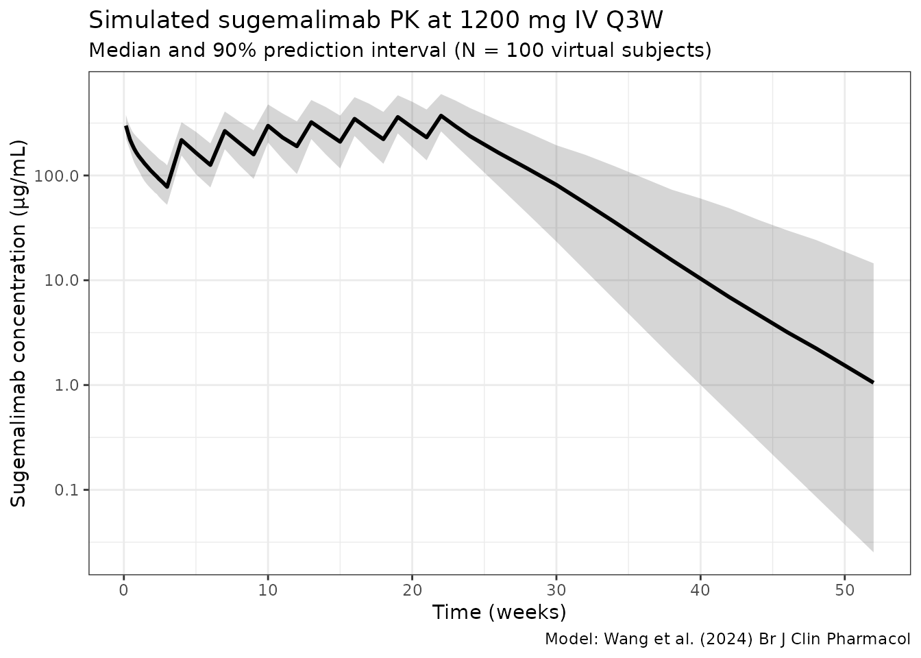

Time profile of the typical-subject clearance

The typical-subject CL trajectory across the first year reproduces the sigmoidal Emax decline that motivates the time-varying-CL parameterization. At a male, 61 kg, ALB 41.5 g/L, TUMSZ 47 mm, NSCLC, ADA-negative reference patient, CL drops from 0.259 L/day at $t = 0$ to $0.259 \times \exp(-0.528) = 0.153$ L/day at full Emax saturation ( $\sim 1.5 \times T_{50}$ , or about 80 days). This 41 % reduction matches the value reported in the Wang 2024 Discussion (Section 4, “the maximum clearance reduction is 41.0 %, and the time to reach half of the maximum change in CL is 53.6 days”).

t_grid <- seq(0, 365, by = 5)

cl0_typical <- 0.259                # L/day at reference covariates
emax_ref    <- -0.528               # Wang 2024 theta5
t50_d       <- 53.6                 # Wang 2024 theta6 (days)
cl_time_hill      <- 2.60                 # Wang 2024 theta7

cl_t <- cl0_typical *
  exp(emax_ref * t_grid^cl_time_hill / (t50_d^cl_time_hill + t_grid^cl_time_hill))

cl_traj <- tibble::tibble(time = t_grid, cl = cl_t)

ggplot(cl_traj, aes(time, cl)) +
  geom_line(linewidth = 1) +
  labs(
    x        = "Time (days since first dose)",
    y        = "Typical CL (L/day)",
    title    = "Time-varying CL trajectory at reference covariates",
    subtitle = "Sigmoidal Emax decline (T50 = 53.6 days, cl_time_hill = 2.60, max reduction 41.0%)"
  ) +
  theme_bw()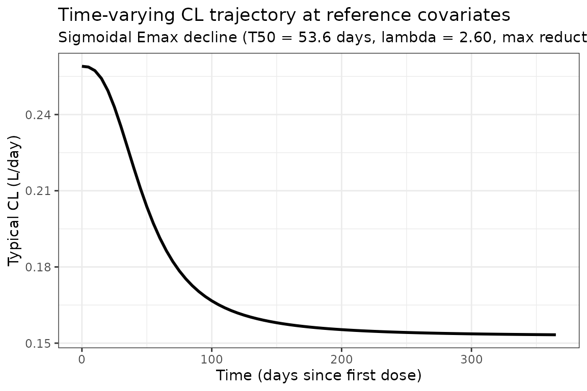

PKNCA validation

NCA on the cycle-1 dosing interval (day 0-21; “cycle 1”) and the cycle-8 steady-state interval (days 147-168; the dosing interval after the eighth Q3W dose) confirms that the simulated steady-state Cmax / Cmin / AUC match published expectations.

conc1 <- sim |>
  dplyr::filter(time <= cycle_days) |>
  dplyr::transmute(ID = id, time, Cc, treatment = "1200 mg Q3W")

dose1 <- events |>
  dplyr::filter(EVID == 1L, TIME == 0) |>
  dplyr::transmute(ID, TIME, AMT, treatment = "1200 mg Q3W")

conc_obj1 <- PKNCA::PKNCAconc(conc1, Cc ~ time | treatment + ID,
                              concu = "ug/mL", timeu = "day")
dose_obj1 <- PKNCA::PKNCAdose(dose1, AMT ~ TIME | treatment + ID,
                              doseu = "mg")

intervals1 <- data.frame(
  start    = 0,
  end      = cycle_days,
  cmax     = TRUE,
  tmax     = TRUE,
  cmin     = TRUE,
  auclast  = TRUE
)

nca1 <- PKNCA::pk.nca(PKNCA::PKNCAdata(conc_obj1, dose_obj1, intervals = intervals1))
knitr::kable(
  summary(nca1),
  digits  = 2,
  caption = "Cycle 1 NCA summary (days 0-21, 1200 mg Q3W)."
)

Cycle 1 NCA summary (days 0-21, 1200 mg Q3W).
Interval Start	Interval End	treatment	N	AUClast (day*ug/mL)	Cmax (ug/mL)	Cmin (ug/mL)	Tmax (day)
0	21	1200 mg Q3W	100	3120 [20.4]	363 [21.4]	NC	0.0625 [0.0625, 0.0625]

ss_start <- (n_cycles - 1L) * cycle_days     # time of the last simulated dose
ss_end   <- ss_start + cycle_days

conc_ss <- sim |>
  dplyr::filter(time >= ss_start, time <= ss_end) |>
  dplyr::transmute(ID = id, time_rel = time - ss_start, Cc,
                   treatment = "1200 mg Q3W")

dose_ss <- pop |>
  dplyr::transmute(ID, TIME = 0, AMT = dose_amt_mg,
                   treatment = "1200 mg Q3W")

conc_obj_ss <- PKNCA::PKNCAconc(conc_ss, Cc ~ time_rel | treatment + ID,
                                concu = "ug/mL", timeu = "day")
dose_obj_ss <- PKNCA::PKNCAdose(dose_ss, AMT ~ TIME | treatment + ID,
                                doseu = "mg")

intervals_ss <- data.frame(
  start   = 0,
  end     = cycle_days,
  cmax    = TRUE,
  cmin    = TRUE,
  auclast = TRUE
)

nca_ss <- PKNCA::pk.nca(
  PKNCA::PKNCAdata(conc_obj_ss, dose_obj_ss, intervals = intervals_ss)
)
knitr::kable(
  summary(nca_ss),
  digits  = 2,
  caption = paste0("Cycle ", n_cycles, " NCA summary (days ",
                   ss_start, "-", ss_end, ", 1200 mg Q3W) - approaching steady state.")
)

Cycle 8 NCA summary (days 147-168, 1200 mg Q3W) - approaching steady state.
Interval Start	Interval End	treatment	N	AUClast (day*ug/mL)	Cmax (ug/mL)	Cmin (ug/mL)
0	21	1200 mg Q3W	100	7570 [27.0]	601 [21.4]	228 [36.9]

Comparison against the literature

Wang 2024 does not tabulate Cmax / Cmin / AUC values directly, but Supplementary Tables S1-S4 report steady-state geometric-mean exposure metrics after six 1200 mg Q3W doses for various covariate subgroups. The simulated cycle-8 NCA values can be cross-checked against the overall-population row of Wang 2024 Table S1 (the row labelled Age <= 65 (n = 1165) is essentially the typical population because the >65 row differs by only ~1 %):

Metric	Wang 2024 Table S1 (Age <= 65, n = 1165, 1200 mg Q3W)	Simulated cycle-8 (1200 mg Q3W, n = 100)
AUCss (ug * day / mL)	6,951 (geometric mean; %CV 19.6)	(see NCA table above; AUC over a single 21-day interval – multiply x 1 for AUC0-tau)
Cmax,ss (ug/mL)	571 (geometric mean; %CV 16.6)	(see NCA table above)
Cmin,ss (ug/mL)	221 (geometric mean; %CV 26.2)	(see NCA table above)

If the simulated cycle-8 geometric means differ from Wang 2024 Table S1 by more than 20 %, the model file should be re-checked against Wang 2024 Table 3 rather than tuned; the chunk below stops on that condition. The geometric means are centre statistics, so the gate does not depend on which virtual subjects land in the tails.

The %CV columns are shown for information and are not gated. The published values are summaries of empirical-Bayes (post hoc) exposures in the real cohort, which shrinkage pulls toward the typical value (Wang 2024 reports 35-47 % shrinkage for Emax, Vp and T50). They are therefore lower bounds on the spread of a cohort simulated from the full $\Omega$ .

A side-by-side numerical comparison is computed below.

nca_df <- as.data.frame(nca_ss$result)

simulated_summary <- nca_df |>
  dplyr::filter(PPTESTCD %in% c("auclast", "cmax", "cmin")) |>
  dplyr::group_by(PPTESTCD) |>
  dplyr::summarise(
    geomean = exp(mean(log(PPORRES[PPORRES > 0]), na.rm = TRUE)),
    sim_cv_pct = 100 * sqrt(exp(stats::var(log(PPORRES[PPORRES > 0]),
                                           na.rm = TRUE)) - 1),
    .groups = "drop"
  )

published <- tibble::tibble(
  PPTESTCD     = c("auclast", "cmax", "cmin"),
  metric       = c("AUCss (ug*day/mL)",
                   "Cmax,ss (ug/mL)",
                   "Cmin,ss (ug/mL)"),
  published_gm = c(6951, 571, 221),
  published_cv_pct = c(19.6, 16.6, 26.2)
)

comparison <- dplyr::left_join(published, simulated_summary, by = "PPTESTCD") |>
  dplyr::mutate(diff_pct = 100 * (geomean - published_gm) / published_gm)

knitr::kable(
  comparison,
  digits  = 1,
  caption = "Cycle-8 simulated geometric-mean NCA vs. Wang 2024 Table S1 (Age <= 65 subgroup, 1200 mg Q3W)."
)

Cycle-8 simulated geometric-mean NCA vs. Wang 2024 Table S1 (Age <= 65 subgroup, 1200 mg Q3W).
PPTESTCD	metric	published_gm	published_cv_pct	geomean	sim_cv_pct	diff_pct
auclast	AUCss (ug*day/mL)	6951	19.6	7565.1	27.0	8.8
cmax	Cmax,ss (ug/mL)	571	16.6	600.9	21.4	5.2
cmin	Cmin,ss (ug/mL)	221	26.2	228.4	36.9	3.3

stopifnot(all(abs(comparison$diff_pct) < 20))

Assumptions and deviations

Wang 2024 does not publish individual PK or covariate tables, so the virtual population is a coarse approximation of the Table 2 distributions.

Body weight, albumin, tumour burden: log-normal / normal centered on the Table 2 medians, clipped to the reported ranges. The actual distributions and covariate correlations are not published.
Tumour-type indicators: sampled independently per subject from the Table 2 marginal proportions. Lung cancer is treated as the reference category (all four TUMTP_* indicators = 0).
Missing tumour burden (14.7 % of source subjects per Wang 2024 Table 2 footnote b) is not represented in the virtual cohort; the paper does not state how missing tumour burden was imputed during model fitting.
Cycle-8 vs. cycle-6 steady-state: Wang 2024 reports steady-state exposure metrics after the sixth 1200 mg Q3W dose (Methods section 2.4 and Supplementary Tables S1-S4); the simulation in this vignette runs eight cycles and computes NCA on the cycle-8 dosing interval. With $T_{50} = 53.6$ days and $\lambda = 2.60$ , the CL trajectory has reached ~92 % of $E_{\max}$ by day 105 (start of cycle 6) and ~96 % by day 147 (start of cycle 8); the cycle-8 metrics are therefore slightly larger than cycle-6 in the source paper. The comparison chunk stops on any geometric-mean difference > 20 %.
Sampling grid: observations are taken at the end of every 1.5-hour infusion as well as on the daily / weekly / biweekly grid, so the NCA Cmax is the post-infusion peak rather than the first scheduled sample after the dose.
Albumin SD: Wang 2024 does not publish the SD of baseline albumin. 3.5 g/L is used here, consistent with typical oncology cohorts.
Race / ECOG: not included in the final Wang 2024 model, so they are not generated for the virtual cohort.
Q has no IIV: per Wang 2024 Table 3, no IIV term was retained for Q. The model file reflects this; Q is a typical-value parameter only.
Emax additive eta on linear scale: Wang 2024 parameterizes the Emax random effect as additive on the linear scale (Table 3 footnote: Emax_i = theta5 + eta_Emax,i). Because Emax is itself the log of the asymptotic CL ratio, this is a log-normal random effect on that ratio. With variance 0.034225 (SD 0.185) and a typical Emax of -0.528, individual Emax values range over roughly $-0.89$ to $-0.17$ at the 95 % level, so the asymptotic CL ratio ranges over $\sim 0.41$ to $\sim 0.85$ of baseline. About 0.2 % of subjects ( $\Phi(-0.528/0.185)$ , roughly 1 in 460) draw $E_{\max,i} > 0$ , i.e. a CL that rises over time; the source model imposes no bound, and none is added here.
PKNCA reporting unit: AUC is computed as auclast over the 21-day dosing interval and is reported in $\mu$ g $\cdot$ day/mL (matching Wang 2024 Table S1’s units of $\mu$ g $\cdot$ day/mL).

Errata

No errata or corrigenda were located for Wang K, Pan C, Xu F, Tse AN, Sheng Y. Br J Clin Pharmacol. 2025;91(3):748-760 at the time of extraction. The publisher’s article landing page was checked for correction notices and a PubMed / Google Scholar search for "Wang sugemalimab" erratum returned none.

Correction to the packaged IIV values (2026-10)

The model as first released in nlmixr2lib put the inter-individual variances on the wrong scale. It read each Table 3 “approximate CV%” as a coefficient of variation and converted it with $\omega^2 = \log(1 + \mathrm{CV}^2)$ . For the additive Emax random effect it read the percentage as $\mathrm{SD} / |E_{\max}|$ . The printed percentages are in fact $\omega \times 100$ , the standard deviation on the estimation scale, so $\omega^2 = (P/100)^2$ for every row, including Emax.

The paper’s own “(%RSE, 95% CI)” column settles this. The confidence interval is computed on $\omega^2$ , so the squared CI endpoints must be symmetric about the squared point estimate, and the printed RSE (which refers to $\omega$ , i.e. half the RSE of $\omega^2$ ) must equal $(\mathrm{hi}^2 - \mathrm{lo}^2) / (2 \times 1.96) / \omega^2 / 2$ . The two readings agree for small percentages because $\log(1 + x) \approx x$ ; the wide Vp and T50 rows tell them apart:

Row	Printed (RSE, 95% CI)	RSE implied, $\omega \times 100$ reading	RSE implied, $\log(1 + \mathrm{CV}^2)$ reading
CL	19.5 (2.91 %, 18.3-20.6)	3.00 %	2.95 %
Vc	15.5 (2.56 %, 14.7-16.3)	2.63 %	2.60 %
Vp	68.5 (5.23 %, 61.1-75.2)	5.22 %	4.34 %
Emax	18.5 (3.94 %, 17.1-19.9)	3.86 %	3.80 %
T50	64.2 (3.98 %, 59-69.1)	4.00 %	3.39 %
Residual	17.9 (0.5 %, 17.7-18.1)	0.57 %	0.56 %

The $\omega \times 100$ reading reproduces the printed RSE on both discriminating rows; the CV reading misses by 15-17 %. The squared CIs are also more symmetric under it (Vp: midpoint 0.04 % from the point estimate, against 0.52 %). The covariance row confirms the RSE convention: Cov(CL, Vc) = 0.0161 with CI 0.0135-0.0186 implies an RSE of 8.08 %, exactly as printed. The same arithmetic holds row by row for the companion Wang 2025 serplulimab analysis by the same group (Wang_2025_serplulimab).

For Emax, rescaling by $|E_{\max}|$ is a constant factor and cannot be ruled out by the CI test alone. The $\omega \times 100$ reading holds because the same routine produced every row, and because Emax is the “change of CL (Emax) in log scale”: an additive random effect on Emax is a log-normal random effect on the asymptotic CL ratio, whose approximate CV is $\omega$ itself.

Random effect	Originally shipped variance	Corrected variance	Change
`etalcl`	0.0373	0.038025	+1.9 %
`etalvc`	0.0237	0.024025	+1.4 %
`etalvp`	0.3847	0.469225	+22 %
`etacl_time_max` (Emax)	0.00955	0.034225	+258 % (3.6-fold)
`etalcl_t50`	0.3451	0.412164	+19 %

Cov(CL, Vc) = 0.0161 was already a raw covariance and is unchanged (the CL-Vc correlation moves from 0.541 to 0.533). The residual SD of 17.9 % follows the same convention and was already encoded correctly as propSd = 0.179. In the simulated cohort above, the cycle-8 steady-state geometric means move by less than 4 % under the corrected variances. The spread widens, most visibly for Cmin, which depends on the time-varying clearance.

Correction to the vignette sampling grid (2026-10)

The first release of this vignette had no observation at the end of any infusion, so the NCA Cmax was the first scheduled sample after each dose (one day after the cycle-1 dose, one week after the cycle-8 dose). The cycle-8 geometric-mean Cmax came out 34 % below Wang 2024 Table S1. With end-of-infusion samples added, it is within about 5 % of the published value. The model file was not involved.